Noisy Inputs: The Jittery Sensor
Two lightweight ML classifiers – a decision tree and a multilayer perceptron – trained on readings from an ultrasonic sensor fail due to a dataset shift caused by the change of the train's shape. The experiment demonstrates the importance of data preprocessing and highlights the need for a critical interpretation of the models' performance metrics.
- Published
Contents
Artifacts
Introduction
Decision Trees (DT) and Multilayer Perceptrons (MLP) are equally applicable to the classification problem of streaming data from a sensor, the former being the preferred solution when the model interpretability matters, the latter being capable of modelling more complex data patterns. Both may fail, however, in the presence of a sensor noise, which must be addressed with data preprocessing, and dataset shift.
Demonstration overview
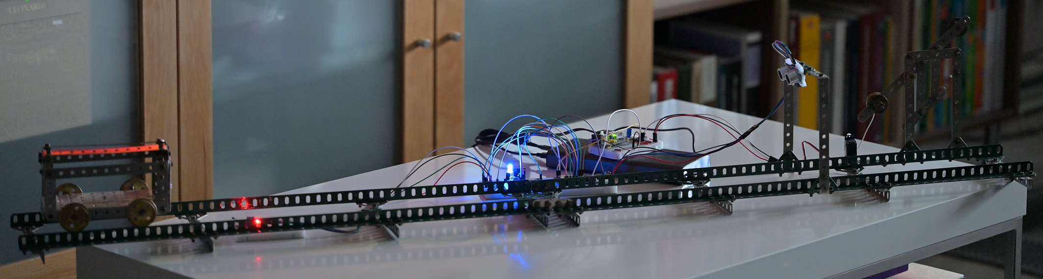
An ESP32 microcontroller is connected to an ultrasonic distance sensor, whose readings define the position of a servo motor attached to the gate. The system models the approaching train detection: the gate remains open if the detected train is braking, otherwise the gate closes.
A model used by the MCU firmware classifies the sensor readings using a pre-trained model. The experiment is conducted with a DT and an MLP. Both models are trained using a model train with a solid vertical front surface. The classification fails when the inference is performed on a different train with a steeply angled front surface or a rotating part with a complex geometry.
Data modelling
1. Feature engineering
Both DTs and MLPs expect a vector with a fixed dimensionality. Because an ultrasonic ping is not sufficient to capture the motion of a train, the input vector should be a rolling window of values calculated from recent distance measurements.
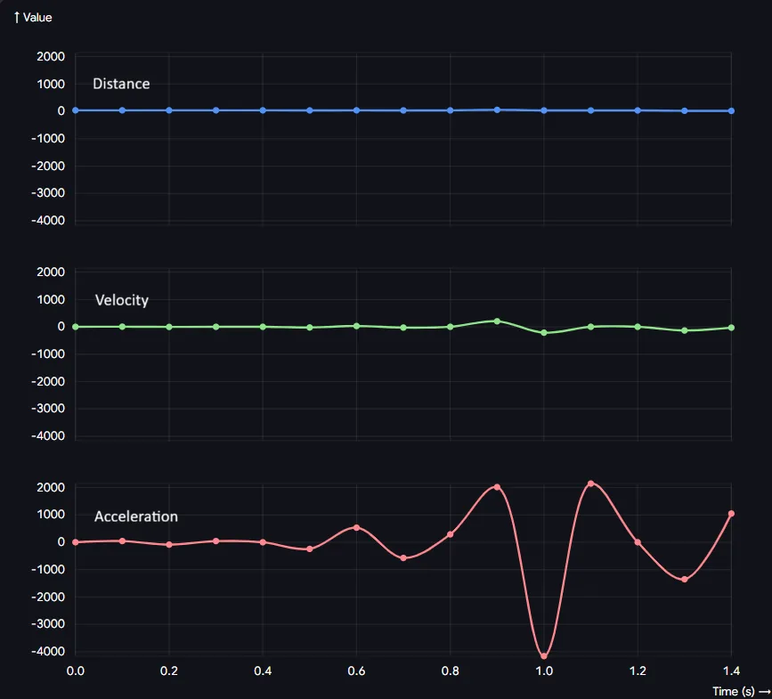
Raw distances lack the context of momentum, crucial for the decision of whether to close the crossing gate, therefore it was decided to include the most recent distance, a number of historical velocities, and a number of historical accelerations in the input vector.
The shape of the resulting dataset:
data = {
    'd_t':   [ 25.07,    32.16,   ...],  # Last distance
    'v_t':   [-40.47,   -10.98,   ...],  # Last velocity
    'v_t_1': [-21.78,   -44.25,   ...],  # Previous velocities...
    'v_t_2': [-31.73,   -16.98,   ...],
    'v_t_3': [-32.58,    -0.17,   ...],
    ...,                                 # (14 values)
    'a_t':   [-15.22,     -3.8,   ...],  # Last acceleration
    'a_t_1': [ -5.14,     0.00,   ...],  # Previous accelerations...
    'a_t_2': [ -1.72,     1.72,   ...],
    ...,                                 # (13 values)
    'target':[     1,        0,   ...]   # 1 = Close gate, 0 = Keep open
}2. Data collection
The data is collected directly from the hardware setup. Because the goal is to demonstrate an AI failure mode caused by dataset shift and noisy inputs, the training data is collected under ideal conditions: a flat, highly reflective object is run past the sensor multiple times. To calculate meaningful velocity and acceleration and achieve high precision, the ultrasonic polling rate is set to roughly 10 readings per second over the timeframe of 1.5 seconds.
Failure modes
At the inference stage, both models displayed a significant amount of false detections, both positive and negative, regardless of the shape of the train. Surprisingly, though, the true positives detection rate rapidly increased for the train with the most irregular shape, although for different reasons and not as an indicator of the model’s success. The analysis of test runs demonstrates the wrong patterns learnt by the models, which resulted in unexpected increased accuracy or unusually high prediction confidence.
The engineering takeaway
This demonstration serves as a vivid lesson on why raw sensor data should never be fed directly into an ML model in the physical world. It visually proves that without data preprocessing techniques – for example, input smoothing (to filter out the noise) used in this experiment, or hysteresis (to prevent the system from rapidly toggling states when hovering near a threshold) – intelligent systems are fundamentally fragile.
Design
The workflow
At any given moment, the system is in one of the three states:
-
STATE_WAITING(blue light) – the system is waiting for the Hall effect sensor to be triggered, indicating that a train is approaching. -
STATE_READING(red light) – the system has received a signal from the Hall effect sensor indicating the approaching train and starts collecting distance readings from the ultrasonic sensor. After receiving 15 readings over 1.5 seconds, a feature array is calculated using the latest distance, 14 rolling velocity values, and 13 rolling acceleration values (28 features in total). After having collected and processed all values, the system transitions into theSTATE_ACTION. -
STATE_ACTION(green light) – depending on the current operation mode, the system acts on the collected data. In theMODE_COLLECTION, the features are printed in the Serial Monitor as a CSV string, where it is intercepted by a COM port listener which saves the data to a file. In theMODE_INFERENCE, the ML model is invoked with the collected data to infer the target gate position (open or closed). After performing the action, the system is listening to theRESETbutton press, which returns it to theSTATE_WAITING.
A single hardware setup is used for the training data collection and the subsequent inference.
To achieve that, in the STATE_WAITING the system is constantly polling its current operation
mode (MODE_COLLECTION or MODE_INFERENCE), which then defines the action.
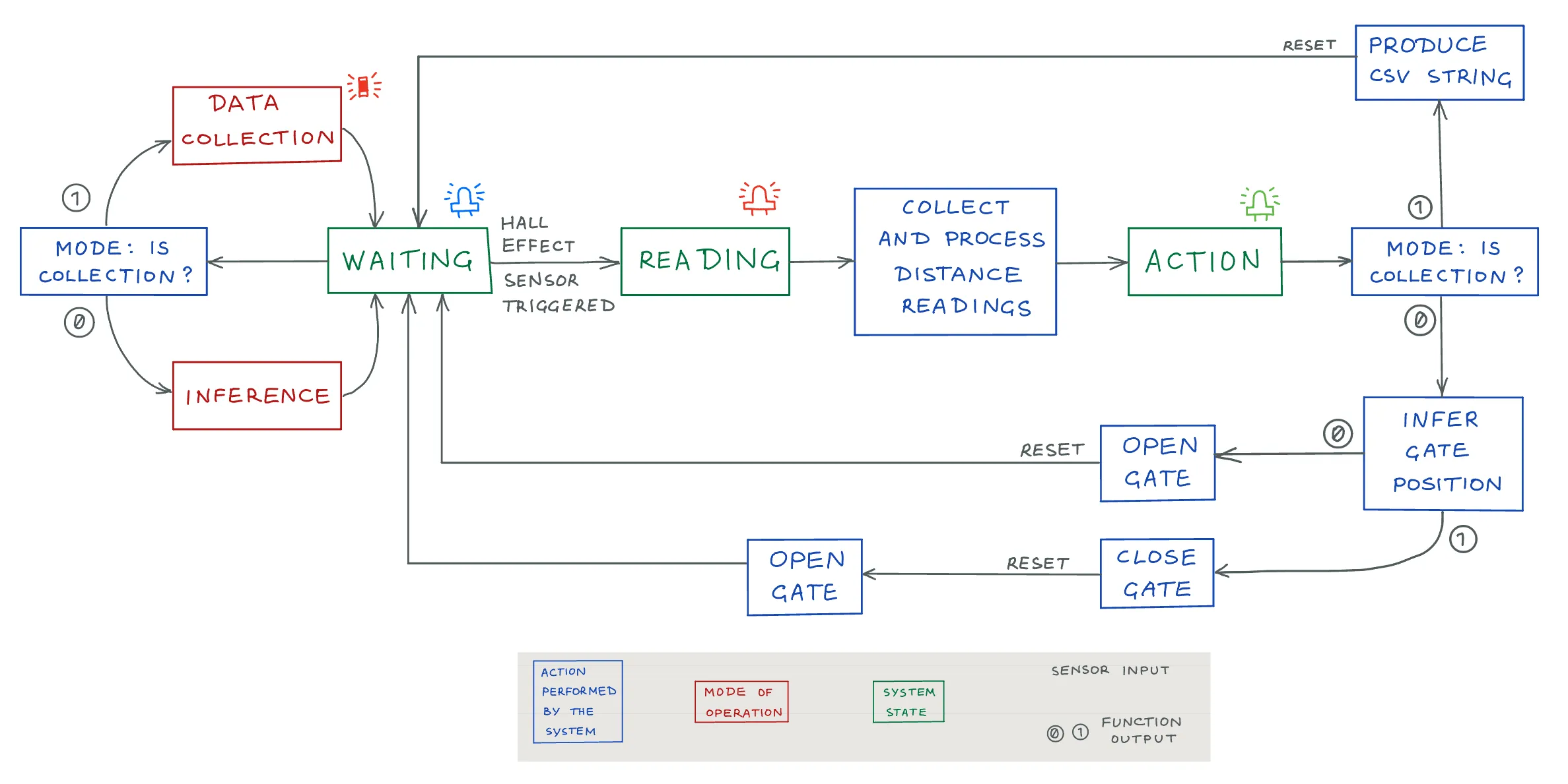
Note: This simplified workflow does not reflect a later addition of handling the distance reading failure. In the
MODE_COLLECTION, a run is discarded if more than half of readings are deemed invalid. In theMODE_INFERENCE, in this situation the gate closes as a fail-safe. In both cases, the state indicator turns yellow, and the system is waiting for a reset.Neither does it show the logic for selecting one of the two inference models (DT and MLP) in the
MODE_INFERENCE, which is controlled by a separate toggle switch.
Theoretical concepts
The problem is structured as a supervised learning task, where objective target labels are provided
alongside the input data. Instead of a conditional action based on the distance reading, i.e.
if (distance < X) close_gate();, two lightweight classifiers that can be deployed on the MCU are
implemented, each with its strengths and trade-offs.
1. Decision Tree (DT)
A Decision Tree makes predictions based on a sequence of “if-then” questions, with nodes performing a test on a specific feature, branches corresponding to the test outcome, and leaves representing the predicted class. The concept of a DT emerged in the 1970s and was further developed in the 1980s as the ID3 algorithm and the CART (Classification and Regression Trees) algorithm.
Despite its representation as a sequense of “if-else” statements, a DT is is considered a machine learning algorithm, because the threshold values are learned from the data. A DT discovers the optimal rules by recursively partitioning the input space into non-overlapping regions using axis-aligned splits and then assessing how “pure” the resulting split is, i.e. how well it separates samples belonging to different classes.
2. Multilayer Perceptron (MLP)
An MLP is a classic type of an artificial neural network consisting of multiple layers of interconnected nodes. The original concept of a single-layer perceptron was suggested in 1958, but practical applications of MLPs became possible in the 1980s with the popularisation of the backpropagation algorithm.
The input layer receives the data, hidden layers perform mathematical transformations, and the output layer produces the final classification. The hyperparameters of individual layers, such as the activation function, are defined by the purpose of the layer.
Trade-offs
DTs are preferred in safety-critical applications for their interpretability, where it’s important to be able to trace a decision back to a clear condition, i.e. where, in case of a failure, the reason for the malfunction must be established. MLPs, on the other hand, while being mathematically difficult to interpret, are highly capable of filtering out noise in the data that can send a DT down a wrong branch, since DTs are built on hard single-feature thresholds. Moreover, DTs produce orthogonal splits of the data that are less suitable for approximating a smooth curve, which would require a deep and complex DT that is likely to overfit. In this case, the non-linearity of an MLP is more helpful for modelling complex data patterns. Finally, instead of 0 (a braking train; keep the gate open) or 1 (the train is not stopping; close the gate), an MLP can produce a confidence score allowing the caller to decide how to act.
| DT | MLP | |
|---|---|---|
| Interpretability | ✔️ | |
| Noise-resistance | ✔️ | |
| Non-linearity | ✔️ | |
| Output | binary | score |
Implementation
Hardware
A note on voltages: The sensors require 5V power, therefore their power pins are connected to the ESP32 USB pin that provides the 5V from the USB connection, rather than to the 3.3V pin.
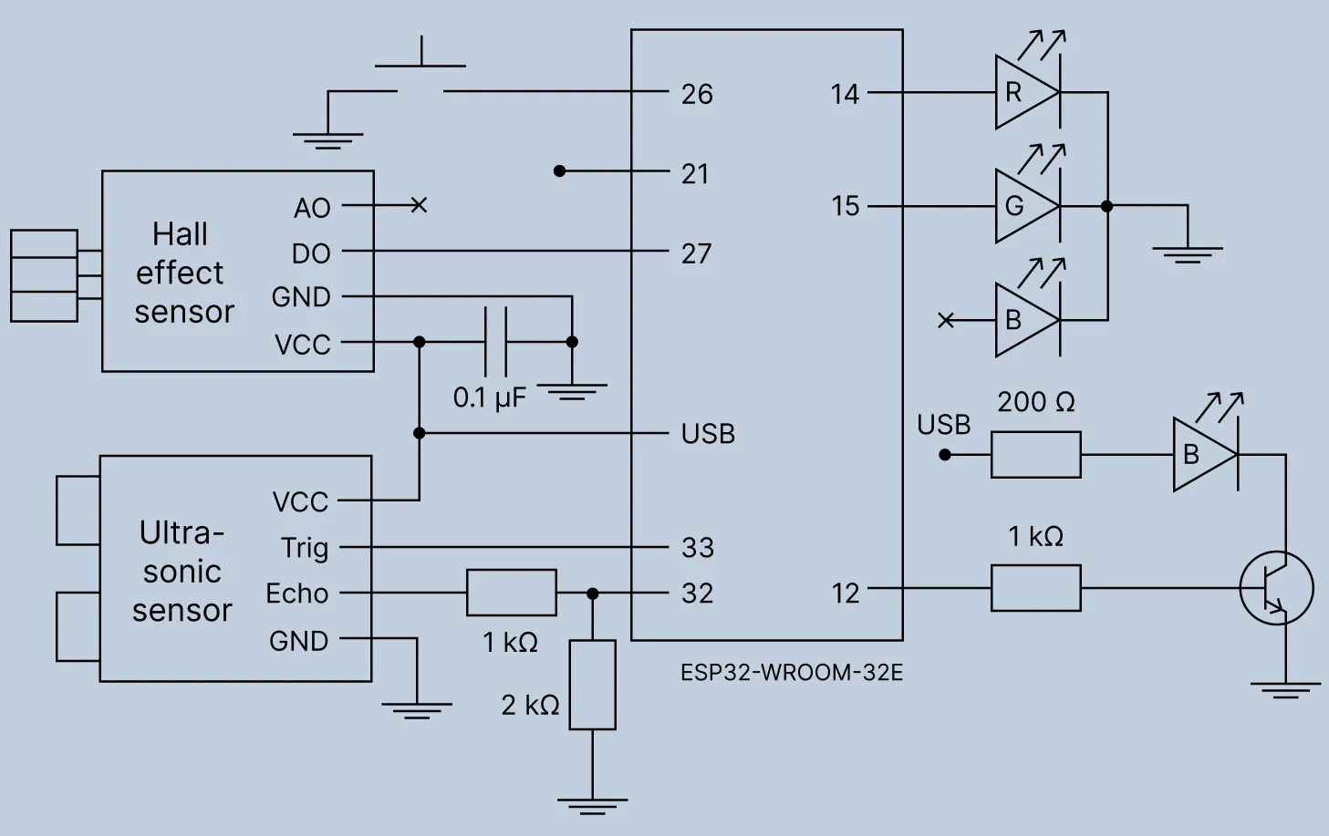
The diagram corresponds to the following wiring plan:
- Hall effect sensor:
VCCESP32 USBGNDESP32GNDDOESP32 GPIO 27
- Push-button (reset):
- Leg 1 ESP32 GPIO 26
- Leg 2 ESP32
GND
- RGB LED (assuming common cathode):
GND(longest leg) ESP32GND- Red leg 330 resistor ESP32 GPIO 14
- Green leg 330 resistor ESP32 GPIO 15
- HC-SR04 ultrasonic sensor:
VCCESP32 USBGNDESP32GNDTRIGESP32 GPIO 33ECHOvoltage divider* ESP32 GPIO 32
* The voltage divider is implemented by placing a 1k resistor between
ECHOand GPIO 32, and a 2k resistor from GPIO 32 toGNDto drop the 5V signal to 3.3V.
The blue LED
The three LED colours in the RGB LED use different semiconductor materials, each with its own minimum forward voltage (), the blue LED’s being the highest (typically around 3 V). With the ESP32 GPIO outputting 3.3 V, the voltage left over for the 150 current-limiting resistor on the breakout board does not produce sufficient current for the light to be visible.
Solution 1: Driving the blue channel via a transistor
One solution is to drive the blue light from the 5 V (USB) pin through an NPN transistor (BC547 B331):
5V ──[ R_ext 100Ω ]──┬──[ 148Ω board ]──[ Blue LED ]──GND (common cathode)
                BC547 collector
                BC547 emitter ────────── GND
                BC547 base ──[ 1kΩ ]──── GPIO12
The 100 external resistor serves two purposes:
- When NPN is off (LED on): total series resistance . This results in the LED current being , making the light clearly visible.
- When NPN is on (LED off): the external resistor limits the transistor’s collector current to , well inside the BC547’s 100 mA maximum.
Since this circuit inverts the blue channel (the GPIO HIGH turns the transistor on and
pulls the anode low, turning off the LED), the logic for the blue pin has to be inverted in the code:
void set_rgb_color(int r, int g, int b) {
    gpio_set_level(LED_R, r);
    gpio_set_level(LED_G, g);
    gpio_set_level(LED_B, !b);
}Solution 2 [Used in this project]: A standalone blue LED
The configuration presented in Solution 1 is a shunt switch, or active-low driver, which uses power to keep the light off. A better solution is to abandon the blue channel on the RGB LED and use a separate blue LED. It can be wired using a low-side switch:
5V ──[ Resistor 200Ω ]──[ Blue LED anode ]
                        [ Blue LED cathode]──BC547 collector
                                             BC547 emitter ────── GND
                                             BC547 base ──────────[ 1kΩ ]──── GPIO12
In this setup, the code is reverted back to the normal gpio_set_level(LED_B, b),
as the HIGH turns the transistor on, which connects the LED to ground, turning it on.
Connecting the servo motor
In hobbyist electronics, such as tutorials for Arduino, motor connection schemes may be simplified, avoiding external power supplies and smoothing out voltage drop with a capacitor placed in parallel with the motor. For a high-performance chip equipped with Wi-Fi and Bluetooth, however, this solution is not sufficient to prevent the brownout and protect the board’s voltage regulator or the computer’s USB port in case of stalling.
To stabilise the system, a separate 5V power supply is provided to the servo motor,
and the GND is shared between the motor and the rest of the circuit.
Note that, due to a high internal resistance, a 9V NiMH block battery is not sufficient for providing current to a servo motor. More appropriate options are 4 AA batteries in series outputting 6V, a USB power bank, or a wall-plug AC-to-DC 5V adapter capable of at least 1 Amp or 2 Amps.
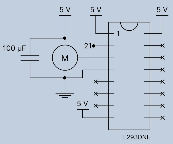
A level shifter
The ESP32 outputs 3.3V on its GPIO pins, which lies below the 3.5V that is considered HIGH
by a 5V servo motor. A dedicated logic level shifter boosts the 3.3V PWM signal to the 5V
necessary for the motor’s stable work. A L293DNE motor driver, though intended to be used with
heavy DC motors, still separates the input logic from the output voltage, functioning as a unidirectional
logic level booster.
Out of the four available channels, only channel 1 is used. Pin 1 being the top-left pin when the L293DNE’s notch is facing UP, the wiring is:
- Pin 1 (
1,2 EN): 5V (enable the left side of the chip) - Pin 2 (
1A/ Input 1): ESP32 GPIO 21 (the 3.3V PWM signal IN) - Pin 3 (
1Y/ Output 1): servo signal wire (the boosted PWM signal OUT) - Pin 4 (
GND): common ground (ESP32 + power supply) - Pin 8 (
VCC2/ motor power): 5V (the voltage the chip pushes to the output pin) - Pin 16 (
VCC1/ logic power): 5V (5V supply for internal logic translation)
Power decoupling
To further reduce the noise on the Power line, a “decoupling” capacitor of 0.1µF is connected across
the power pins of the Hall sensor, and a larger capacitor (100 µF) is placed across the power and GND rails
of the the power module to absorb power spikes created by the servo.
Software
The project’s software comprises the firmware written in C++, including converted DT and MLP models, and a number of Python scripts for constructing the models and gathering data during the training and the test runs.
For the firmware, C++ was chosen over MicroPython or CircuitPython for the following reasons:
-
To calculate velocity and acceleration, highly accurate time deltas from the ultrasonic sensor are required. MicroPython runs an interpreter and a garbage collector and, if the garbage collector pauses execution for a few milliseconds while the signal is travelling, the distance reading will spike, distorting the data.
-
The Python interpreter takes up a significant share of the ESP32’s memory, potentially limiting the size or the number of the models that can be run on the MCU in parallel.
Project setup
The usage of the TensorFlow Light library for creating the “compact” version of the MLP prompts implementing the firmware as a PlatformIO project.
While the Arduino framework is a sensible choice for a simple project with two sensors and a servo, the ESP-IDF framework is used instead to have more control over the hardware, to be able to run C++ ML models natively, and to achieve higher precision of sensor readings:
[env:featheresp32]
platform = espressif32
board = featheresp32
framework = espidfFor Python scripts that process data and build the models, a uv environment is set up with the necessary dependencies:
[project]
dependencies = [
    "pyserial",
    "micromlgen",
    "tensorflow",
    "pandas",
    "scikit-learn"
]pyserialis used to read the data from the COM port during the data collection phase and testing and save it to a file.micromlgenis used to convert the trained DT model into C++ code that can be included in the firmware.tensorflowis used to build and train the MLP model.pandasandscikit-learnare used for data processing and building the DT model.
Firmware architecture
The firmware is structured as a state machine, where the system transitions between states based on sensor inputs and internal timers.
In the main loop, the system state and the mode of operation are monitored using the corresponding enums:
typedef enum {
    MODE_COLLECTION,
    MODE_INFERENCE
} system_mode_t;

typedef enum {
    STATE_WAITING,
    STATE_READING,
    STATE_ACTION
} system_state_t;Two toggle switches define the current mode of operation,
system_mode_t read_mode_from_toggle() {
    // Poll Toggle Switch (LOW = Collection, HIGH = Inference)
    if (gpio_get_level(TOGGLE_GPIO) == 0) {
        gpio_set_level(BUILTIN_LED, 1); // Red LED ON
        return MODE_COLLECTION;
    } else {
        gpio_set_level(BUILTIN_LED, 0); // Red LED OFF
        return MODE_INFERENCE;
    }
}and the model used for inference:
inference_model_t read_inference_model_from_toggle() {
    // LOW selects the DT, HIGH selects the MLP.
    return gpio_get_level(MODEL_SELECT_GPIO) == 0 ? INFERENCE_MODEL_DT : INFERENCE_MODEL_MLP;
}Data collection and feature engineering
The function read_distance_cm() is responsible for reading the distance from the ultrasonic sensor.
It sends a trigger pulse to the sensor, waits for the echo, and calculates the distance
based on the time it takes for the echo to return. The function also includes a timeout mechanism
to handle cases where the sensor fails to provide a valid reading.
float read_distance_cm() {
    gpio_set_level(TRIG_GPIO, 1);
    ets_delay_us(10);
    gpio_set_level(TRIG_GPIO, 0);

    int64_t start_time = esp_timer_get_time();
    int64_t timeout = start_time + 30000;

    while(gpio_get_level(ECHO_GPIO) == 0 && esp_timer_get_time() < timeout);
    int64_t echo_start = esp_timer_get_time();

    while(gpio_get_level(ECHO_GPIO) == 1 && esp_timer_get_time() < timeout);
    int64_t echo_end = esp_timer_get_time();

    int64_t duration = echo_end - echo_start;
    // If the loop broke because it hit the timeout limit, the reading is invalid
    if (duration <= 0 || echo_end >= timeout) return -1.0;

    // Speed of sound is 343 m/s -> 0.0343 cm/µs; divide by 2 for round trip.
    return (duration * 0.0343) / 2.0;
}In the main loop, the distance readings validity is checked to guard against two failure modes:
- the reading falls outside the empirically established range of 1 cm to 70 cm, and
- the sensor times out, which is indicated by the
read_distance_cm()function returning -1.0 (this error code falls outside the valid range and does not require special handling).
”Hold Last Valid” filter
Invalid readings are not simply discarded leaving a gap in the data, but are replaced with the last valid reading (or the inital 70 cm distance if no valid reading has been received yet). Because the train is moving linearly and is small (100ms), holding the last valid frame keeps the velocity and acceleration values stable without causing extreme spikes.
Omitted values, however, highlight another signal processing problem: numerical differentiation amplifies noise. A sudden spike in the distance reading, even if it is a single outlier, can cause a large velocity spike, which in turn causes an even larger acceleration spike. This can send a DT down a wrong branch or cause an MLP to produce an incorrect prediction with high confidence. This is avoided by using a median filter over a sliding window of 3 readings (duplicating the nearest neighbour for edges), which smoothes out outliers without distorting the real movement of the train.
static float median3f(float a, float b, float c) {
    if ((a >= b && a <= c) || (a >= c && a <= b)) return a;
    if ((b >= a && b <= c) || (b >= c && b <= a)) return b;
    return c;
}Building the models
The project compares Decision Trees, which offer transparent and auditable logic, against Multilayer Perceptrons that excel at filtering sensor noise. Both models must be deployed on the MCU to ensure real-time inference, which requires converting them into C++ code.
Decision Tree
The DT model is buit and trained using the scikit-learn library, and then converted into C++ code using the micromlgen library,
which generates a series of nested “if-else” statements that can be included in the firmware.
from sklearn.tree import DecisionTreeClassifier, export_text
from micromlgen import port

# X and y are the feature matrix and target vector from the training dataset,
# extracted from the collected data stored in the .csv file by the Pandas library.

tree_model = DecisionTreeClassifier(max_depth=3, random_state=42)
tree_model.fit(X, y)

header_path = os.path.join('include', 'gate_model.h')
with open(header_path, 'w', encoding='utf-8') as header_file:
header_file.write(port(tree_model))The model exported as a series of nested “if-else” statements, remarkably only including the current distance and velocities (mostly the first and the last registered), but none of the accelerations. The resulting DT can be interpreted in the following fashion:
IF current velocity <= -2.06 cm/s (the train is moving slowly):
|--- IF velocity from 6 readings ago <= -1.80 (the train was moving faster):
| |--- IF first registered velocity <= 0.86:
| | |--- THEN: OPEN GATE (the recent motion history matches a safe pattern)
| | |
| | ELSE (first velocity > 0.86):
| | |--- THEN: CLOSE GATE (the motion history points to a riskier approach pattern)
| |
| ELSE (velocity from 6 readings ago > -1.80):
| |--- IF current distance <= 31.245 cm:
| | |--- THEN: CLOSE GATE (the train is too close)
| | |
| | ELSE (current distance > 31.245 cm):
| | |--- THEN: OPEN GATE (the train is farther away, so the model allows opening)
|
ELSE (current velocity > -2.06):
|--- IF first registered velocity <= -0.775:
| |--- IF current distance <= 36.06 cm:
| | |--- THEN: OPEN GATE (despite the train being close, it's treated as safe enough)
| | |
| | ELSE (current distance > 36.06 cm):
| | |--- THEN: CLOSE GATE (conservative at larger distance -- the movement can change)
| |
| ELSE (first registered velocity > -0.775):
| |--- IF first registered velocity <= 0.425:
| | |--- THEN: OPEN GATE (the train slowed down during the measurement window)
| | |
| | ELSE (first registered velocity > 0.425):
| | |--- THEN: CLOSE GATE (anomalous pattern)
Note: The “current velocity” is actually the velocity from the previous pair of readings – the term “current” is used for simplicity. Also note that positive velocity values are anomalous, as they indicate the train moving away from the sensor, which is not expected in this scenario.
Multilayer Perceptron
The MLP’s hyperparameters define the model’s architecture with the following considerations in mind: The input layer is locked at the number of features (1 + 14 + 13 = 28), the output layer is locked at 1 (the confidence score for closing the gate), and the hidden layer(s) are defined based on the complexity of the data patterns and the need to avoid overfitting.
1. Network topology
The network topology is chosen out of the following options:
-
Option A: Shallow and wide. A single hidden layer with a sufficient number of neurons may be enough to approximate most continuous functions. It calculates quickly and is less prone to overfitting. However, such a NN may struggle with combining velocity and acceleration features into a highly complex braking pattern.
-
Option B: Deep and funnelled. Multiple hidden layers with a decreasing number of neurons can capture more complex patterns. The first layyer finds basic patterns, like high velocity, and the subsequent layers combine these patterns into higher-order concepts, like high velocity and sufficient negative acceleration may indicate a braking train. Funnelling the neuron count helps to distill the information down to the most critical features before making a decision. However, this architecture is more prone to overfitting on the small dataset of 1000 samples and, with a larger number of weights, requires longer training.
2. Activation function
The purpose of the activation function is to introduce non-linearity into the model, allowing it to learn complex patterns. For hidden layers, the ReLU (Rectified Linear Unit) activation function is a common choice due to its simplicity and efficiency. For the output layer, the mathematically correct choice is the sigmoid function, since the model is supposed to produce a confidence score.
A note on the selection of the activation function for hidden layers:
ReLU being the industry default, other alternatives are worth considering.
- Leaky ReLU addresses the “dead neuron” problem, where neurons can become inactive and stop learning entirely. Instead, it assigns a small non-zero gradient to the negative input values, allowing the network to continue learning even when some neurons are not activated.
- Tanh (Hyperbolic Tangent) is a smoother activation function that outputs values between -1 and 1, which can be beneficial when data is centred around zero. In the case of deep networks, however, this function suffers from the “vanishing gradient” problem, where for very high or very low inputs the curve goes flat and the learning halts.
- ELU (Exponential Linear Unit) or GELU (Gaussian Error Linear Unit) offer a smoother curve than ReLU, which in case of modelling complex physical reality of a moving body can help us to achieve maximum accuracy. Both are significantly slower in training, especially for large networks, but even with the small MLP they can slow down the real-time inference when deployed on the MCU.
In practice, the standard ReLU is a sound choice that shows sufficiently good performance most of the time. If the network struggles to learn, the LeakyReLU is a sound alternative, and for a shallow network using ELU/GELU or Tanh can be considered to further increase the accuracy, if needed.
3. Regularisation
In the presence of the sensor noise, regularisation is the way to diminish the model’s reliance on any single feature. This can be achieved by adding a dropout layer that randomly sets a pre-defined fraction of the input units to 0 during each training pass. Dropout increases the system’s robustness at the cost of a longer training time.
4. Optimiser and loss function
The binary cross-entropy loss function penalises the model for being confidently wrong, which is an appropriate measure for a model that outputs a probability (the confidence score). The Adam optimiser automatically adjusts the learning rate, taking large steps at the early training stages and smaller steps as it approaches a minimum.
5. Normalisation
Feeding raw numerical values for both distances (tens of centimetres), velocities (negative centimetres per second), and acceleration (both positive and negative centimetres per second squared) will certainly break the network. This problem is addressed by normalising the input data by scaling all features to a similar range.
For normalising the training data, the built-in Normalization layer is sufficient, as it performs the Z-score standardisation
by shifting the data so that the mean value of every feature is 0 with a standard deviation of 1:
normalizer = tf.keras.layers.Normalization(axis=-1)
normalizer.adapt(X_train)

model = Sequential([
    normalizer,
    # ... (hidden layers and output layer) ...
])After deploying the model on the MCU, the same transformation must be applied to the input data before feeding it into the model. The mean () and the standard deviation () values must be calculated using historical data and stored separately, so that the input vector could be normalised using those exact scaling parameters:
norm_layer = next(l for l in model.layers if isinstance(l, tf.keras.layers.Normalization))
norm_mean = norm_layer.mean.numpy().flatten()  # Stored as mlp_norm_mean in the firmware
# Normalization computes (x - mean) / sqrt(variance + epsilon); epsilon = 1e-3 by default.
norm_std = np.sqrt(norm_layer.variance.numpy().flatten() + 1e-3) # Stored as mlp_norm_std in the firmwareThe norm_mean and norm_std arrays are then used at the inference stage:
// Normalise: x_n[i] = (x[i] - mean[i]) / std[i]
float xn[MLP_INPUT];
for (int i = 0; i < MLP_INPUT; i++) {
    xn[i] = (x[i] - mlp_norm_mean[i]) / mlp_norm_std[i];
}The resulting MLP architecture
With the small dataset of about 800 training samples, dense layers of modest width are sufficient to capture the patterns in the data without overfitting.
The final architecture is as follows Normalization → Dense(32, relu) → Dropout(0.3) → Dense(16, relu) → Dropout(0.2) → Dense(1, sigmoid):
    model = Sequential([
        normalizer,
        Dense(32, activation='relu'),
        Dropout(0.3),
        Dense(16, activation='relu'),
        Dropout(0.2),
        Dense(1, activation='sigmoid'),
    ])

    model.summary()

    model.compile(
        optimizer='adam',
        loss='binary_crossentropy',
        metrics=['accuracy'],
    )

    early_stop = tf.keras.callbacks.EarlyStopping(
        monitor='val_loss',
        patience=15,
        restore_best_weights=True,
    )

    model.fit(
        X_train, y_train,
        epochs=150,
        batch_size=32,
        validation_data=(X_test, y_test),
        callbacks=[early_stop],
        verbose=1,
)The normalisation is adapted on the training data, as described above, and included into the TFLite binary. Two dropout layers
at 0.3 and 0.2 are sufficient to prevent overfitting without affecting accuracy. The early stopping recovers the best checkpoint
when val_loss plateaus for 15 epochs, showing that the model has reached the learning limit on the given dataset.
Porting to the MCU
First, the Keras model must be converted to the TensorFlow Lite format. The applied optimisation converts 32-bit floating point weights to 8-bit integers, which is a common practice for deploying models on microcontrollers, as it significantly reduces the model size and inference time with minimal loss in accuracy.
converter = tf.lite.TFLiteConverter.from_keras_model(model)
converter.optimizations = [tf.lite.Optimize.DEFAULT]
tflite_model = converter.convert()

tflite_path = 'mlp_model.tflite'
with open(tflite_path, 'wb') as f:
f.write(tflite_model)The TFLite model can be used in one of two ways:
- Interpreted (preserved for debugging, retraining, or optional transition to TFLite-Micro). The TFLite model is included in the firmware as a byte array, and the TFLite Micro interpreter is used to run inference on the MCU. This approach is more flexible, as it allows for easy updates to the model without changing the firmware code, but it may have a higher inference time due to the overhead of the interpreter:
bytes_list = [f'0x{b:02X}' for b in tflite_model]
    row_size = 12
    rows = [
        '    ' + ', '.join(bytes_list[i:i + row_size])
        for i in range(0, len(bytes_list), row_size)
    ]
    hex_block = ',\n'.join(rows)

    header = f'''#pragma once

#include <stdint.h>

// Auto-generated by mlp.py — do not edit by hand.
// Re-run mlp.py to regenerate after retraining.
static const uint8_t mlp_model_tflite[] = {{
{hex_block}
}};

static const unsigned int mlp_model_tflite_len = {len(tflite_model)};
'''

    header_path = os.path.join('include', 'mlp_model_data.h')
    with open(header_path, 'w', encoding='utf-8') as f:
f.write(header)- Manually ported (used in the firmware). The model is converted into C++ code that directly computes the output based on the input features, without the need for an interpreter. This approach has a much faster inference time, but it requires more effort to implement and update the model:
    norm_layer = next(l for l in model.layers if isinstance(l, tf.keras.layers.Normalization))
    dense_layers = [l for l in model.layers if isinstance(l, tf.keras.layers.Dense)]

    norm_mean = norm_layer.mean.numpy().flatten()
    # Normalization computes (x - mean) / sqrt(variance + epsilon); epsilon = 1e-3 by default.
    norm_std = np.sqrt(norm_layer.variance.numpy().flatten() + 1e-3)

    # Keras stores Dense weights as (in, out).  Transpose to (out, in) so the C forward
    # pass can index as W[j * IN + i] for output neuron j and input i.
    W1, b1 = dense_layers[0].get_weights()   # (28, 32), (32,)
    W2, b2 = dense_layers[1].get_weights()   # (32, 16), (16,)
    W3, b3 = dense_layers[2].get_weights()   # (16,  1), ( 1,)

    def arr_to_c(name, arr, cols=8):
        flat = arr.flatten()
        entries = [f'{v:.8f}f' for v in flat]
        rows = [
            '    ' + ', '.join(entries[i:i + cols])
            for i in range(0, len(entries), cols)
        ]
        return f'static const float {name}[{len(flat)}] = {{\n' + ',\n'.join(rows) + '\n};'

    weights_header = f'''#pragma once

// Auto-generated by mlp.py — do not edit by hand.
// Architecture: Normalization -> Dense({W1.shape[1]}, relu) -> Dense({W2.shape[1]}, relu) -> Dense(1, sigmoid)

#include <stdint.h>

#define MLP_INPUT {W1.shape[0]}
#define MLP_H1    {W1.shape[1]}
#define MLP_H2    {W2.shape[1]}

// Per-feature normalisation: x_norm[i] = (x[i] - mean[i]) / std[i]
{arr_to_c('mlp_norm_mean', norm_mean)}

{arr_to_c('mlp_norm_std', norm_std)}

// Dense layer 1 weights, shape (H1 x INPUT), row-major
{arr_to_c('mlp_w1', W1.T)}

{arr_to_c('mlp_b1', b1)}

// Dense layer 2 weights, shape (H2 x H1), row-major
{arr_to_c('mlp_w2', W2.T)}

{arr_to_c('mlp_b2', b2)}

// Output layer weights, shape (H2,), and scalar bias
{arr_to_c('mlp_w3', W3.flatten())}

static const float mlp_b3 = {float(b3[0]):.8f}f;
'''

    weights_path = os.path.join('include', 'mlp_weights.h')
    with open(weights_path, 'w', encoding='utf-8') as f:
f.write(weights_header)The arrays corresponding to the MLP layers are then used in the inference function predicting the gate action:
#include "gate_model_api.h"
#include "mlp_weights.h"
#include <cmath>
#include "esp_log.h"

static const char* TAG = "MLP";

// Feature vector layout matches fill_feature_vector in gate_model.cpp:
//   x[0]      = distance
//   x[1..14]  = v[0]..v[13]   (earliest → most recent)
//   x[15..27] = a[0]..a[12]   (earliest → most recent)
//
// mlp.py reverses the CSV column order when building the training set so these
// positions are consistent between training and inference.

extern "C" bool predict_gate_action_mlp(float distance, float* v, float* a) {
    // Build raw feature vector
    float x[MLP_INPUT];
    x[0] = distance;
    for (int i = 0; i < 14; i++) x[1 + i]  = v[i];
    for (int i = 0; i < 13; i++) x[15 + i] = a[i];

    // Normalise: x_n[i] = (x[i] - mean[i]) / std[i]
    float xn[MLP_INPUT];
    for (int i = 0; i < MLP_INPUT; i++) {
        xn[i] = (x[i] - mlp_norm_mean[i]) / mlp_norm_std[i];
    }

    // Dense(H1, relu)
    float h1[MLP_H1];
    for (int j = 0; j < MLP_H1; j++) {
        float s = mlp_b1[j];
        for (int i = 0; i < MLP_INPUT; i++) {
            s += mlp_w1[j * MLP_INPUT + i] * xn[i];
        }
        h1[j] = s > 0.0f ? s : 0.0f;
    }

    // Dense(H2, relu)
    float h2[MLP_H2];
    for (int j = 0; j < MLP_H2; j++) {
        float s = mlp_b2[j];
        for (int i = 0; i < MLP_H1; i++) {
            s += mlp_w2[j * MLP_H1 + i] * h1[i];
        }
        h2[j] = s > 0.0f ? s : 0.0f;
    }

    // Dense(1, sigmoid)
    float logit = mlp_b3;
    for (int i = 0; i < MLP_H2; i++) {
        logit += mlp_w3[i] * h2[i];
    }
    float confidence = 1.0f / (1.0f + expf(-logit));

    ESP_LOGI(TAG, "confidence=%.4f -> %s", confidence, confidence >= 0.5f ? "CLOSE" : "OPEN");
    return confidence >= 0.5f;
}Failure modes
To test the models, a series of experiments was conducted using three types of trains – regular, irregular, and plow – and their results were saved to log files.
For analysis, only the distance readings were saved to logs, without the velocity and acceleration features that were derived from the distance readings in the training data and during inference.
Train types
The regular train has a solid vertical front panel covered with paper for the optimal reflection of the ultrasonic signal. This is the type that was previously used for training the models.
The irregular train has the front wall tilted backwards, imitating a high-speed train. We expect that the alternative geometry will behave differently under the testing conditions compared to the regular train.
The plow train has a rotary snowplow mounted on its front, rotating rapidly as the train moves. We expect that the motion of the plow that has a complex shape will further distort the ultrasonic signal.
Results
The results of the test runs are summarised in the following table showing the false positive rates (FP%) and true positive rates (TPR%) for both the DT and the MLP models across the three train types:
| DT – negative (FP%) | DT – positive (TPR%) | MLP – negative (FP%) | MLP – positive (TPR%) | |
|---|---|---|---|---|
| Regular | 25% | 19% detected | 16% | 76% detected |
| Irregular | 23% | 13% detected | 10% | 58% detected |
| Plow | 18% | 65% detected | 27% | 70% detected |
1. DT
At the first glance, the DT’s high false positive rate across all models and the false negative rate above 80% on regular trains looks like the model is simply broken. A closer look at the failure patters, however, reveals more specific patterns.
Many of the false positive runs have completely flat distance sequences, indicating an unchanging distance to the stopped train, which end with a slight drift from the baseline.This uptick in the distance reading (±1–3 cm) may occur due to the train’s motion settling or the sensor’s noise. During the training it may have been captured by a velocity or acceleration feature and learned as a sign of motion.
The distance readings for the positive runs show clean, monotonic drops indicating the train’s approach, but the model fails to see them. The true positive samples it does detect are characterised by (1) rejected samples at the end, which indicates that the train passed the sensor, or (2) a partial recovery of the approach signal after a peak, e.g. when the distance drops to 14 cm and then bounces back to 23 cm.
The plow surprise
The plow train, which was expected to be the most challenging due to the complex geometry of the rotating front part, actually shows the best performance with a 65% TPR. This points at re-creating a pattern that the model was accidentally trained to recognise.
2. MLP
Many of the MLP’s false negatives on the regular train can be attributed to the overshoot pattern, where the front surface of the train passes the sensor, which then picks up the top of the train which is slightly further away but still within the detection range, indicating the train is moving away from the sensor. The confidence values on these runs are consistently very low, at 0.001 to 0.25, rather than near the 0.5 threshhold, indicating that the model is confidently wrong rather than uncertain. Since false negatives mean that the crossing gate remains open as the train approaches, this is the most dangerous failure mode.

Overall, the MLP model has managed to learn the approach pattern that is shared between all three train types: its 76% detection rateon the regular train and 70% on the plow represent genuine generalisation. The tilted front of the irregular train, however, seems to deflect the signal so that the train appears to be moving away, before the partial recovery at the end of the run. Few of these runs have a very low confidence, indicating that this pattern is not widely represented in the training data.
Conclusion
In addition to the importance of preprocessing the data, the experiment revealed unexpected phenomena, including less than obvious failures caused by physical properties of the system, and an accidental increase in the model’s performance.
Lessons learned
-
The importance of preprocessing. Raw sensor readings should never be fed into a classifier without protecting the downstream model from the physical realities of the system, such as sensor noise, outliers, missing values, or geometry-dependent distortions. The hold last valid strategy and the three-point median filter used in this experiment are minimal interventions capable of preventing the DT from being sent down the wrong branch or the MLP from producing a confident but incorrect prediction by a single outlier.
-
High true positive rates may be a sign of overfitting. The plow train, which was expected to be the most challenging due to its complex geometry, actually shows the best performance with a 65% TPR. This points at re-creating a pattern that the model was accidentally trained to recognise, rather than genuine generalisation.
-
Confidence on false negatives is the most dangerous failure mode. An uncertain model near the 0.5 threshold is recoverable by adjusting the decision boundary or adding a safety margin. The MLP, on the contrary, learned a wrong pattern with conviction, producing confidence values of 0.001 to 0.25 on runs where the gate should close. In a safety-critical context, such confident wrong answers are more dangerous than uncertain ones.
-
Difference in failures: traceability vs adjustability. The DT’s failures are more traceable, as they can be directly linked to specific branches in the tree and the corresponding features. The MLP’s failures, however, are less interpretable, as they result from complex interactions between features and weights. On the other hand, an MLP provides a handle – a confidence score – that can be used to adjust the decision boundary or add a safety margin. In a real deployment, the choice between them would depend on which failure mode is more recoverable given the system’s safety constraints.
Open questions
-
What is the dominant problem: the noise or the dataset shift? A systematic comparison of configurations including different preprocessing techniques and more aggressive smoothing is needed to determine the right amount of intervention required to mitigate the noise without distorting the real movement patterns. It could also reveal the signal distortion is so severe that no amount of preprocessing can compensate for the limitations of the dataset.
-
How should the system handle a previously unseen train during live operation? In the experiment, the idealised geometry of the training object was used to clearly demonstrate the dataset shift. In a real railway, however, new train types are introduced constantly, but retraining requires taking the crossing offline, collecting new data, re-training and redeploying the firmware – a process that is neither fast nor cheap. Moreover, during the transition period the system must remain operational and safe, even if the model’s performance on the new train type is unknown. Options for handling this scenario programmatically include a more conservative decision boundary, a rule-based fallback when the classifier’s confidence falls below a certain threshold, or learning from live operational data.