Introduction

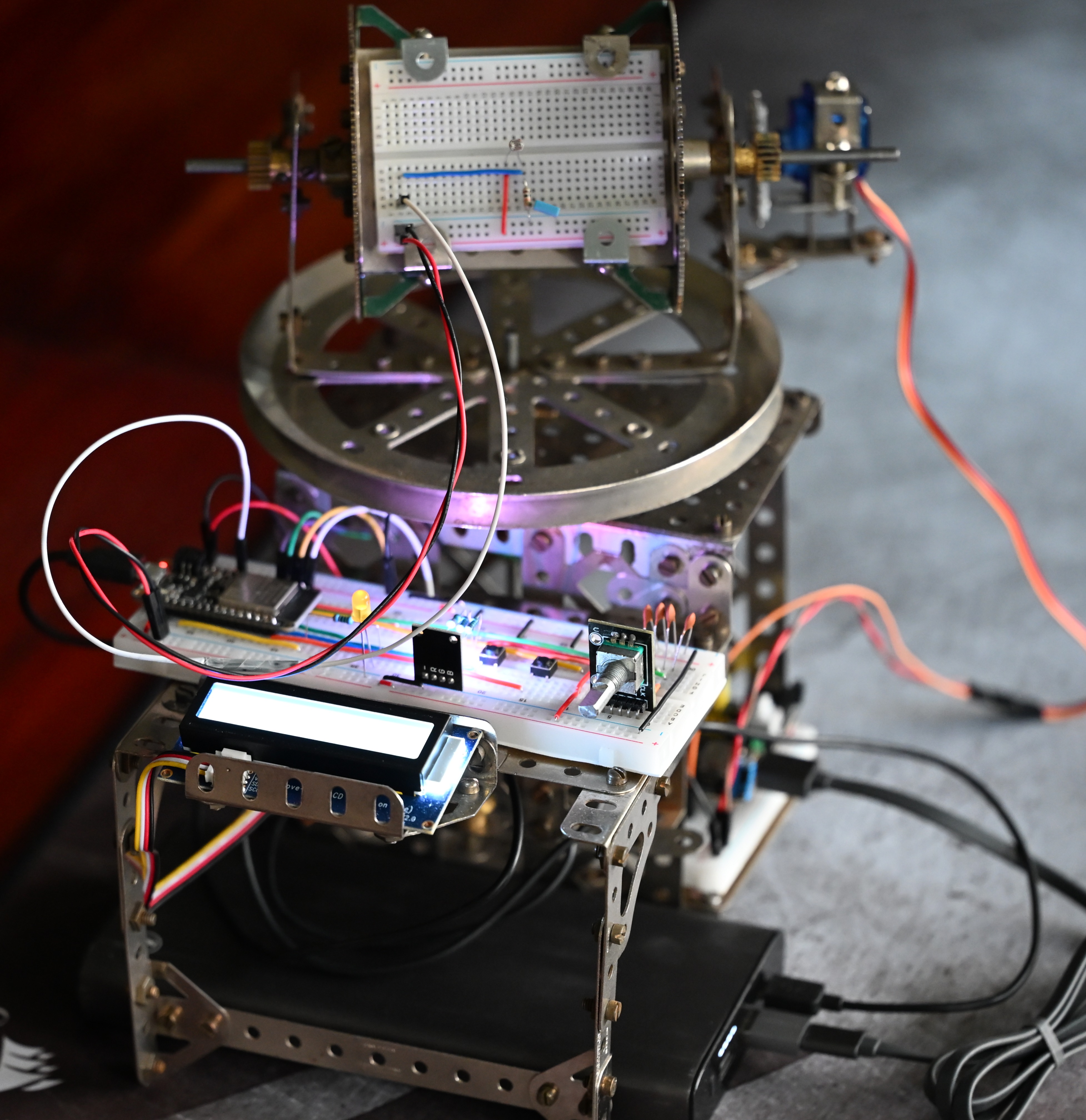
Reward hacking (or specification gaming) is a reinforcement learning phenomenon in which an agent exploits loopholes in the reward function to achieve high rewards without accomplishing the intended task. The Light Seeker project aims to demonstrate reward hacking by a robotic device imitating a solar panel, which is designed to turn towards the light source to maximize its energy intake. However, instead of genuinely seeking the ambient light, the device will learn to find an power indicator on the stationary base of the device. The brightness of the LED indicator exceeds that of the ambient light thanks to its proximity to the sensor, prompting the agent to ignore the environment and lock itself in suboptimal state.

Theoretical foundations

When a measure becomes a target, it ceases to be a good measure. (The Goodhart’s Law re-quoted by Marilyn Strathern)

Framed as a manifestation of Goodhart’s Law, the interaction between the Light Seekeragent and the environment is described in terms of Markov Decision Processes. The solution is implemented using tabular Q-learning, a model-free reinforcement learning algorithm that iteratively learns an optimal policy by updating a table of state-action values (Q-values) based on the rewards received from the environment.

Markov Decision Processes (MDP)

At its core, a Markov Decision Process is a mathematical framework used to describe an environment in reinforcement learning. It relies on the Markov Property, which states that the future depends only on the current state and the action taken, not on the historical sequence of events that preceded it.

Formally, an MDP is defined by a tuple $(S, A, P, R, \gamma)$:

• $S$: A set of states (the state space).
• $A$: A set of actions (the action space).
• $P$: The transition probability function (how likely it is to move from one state to another given an action).
• $R$: The reward function (the immediate return for taking a specific action in a specific state).
• $\gamma$: The discount factor determining the importance of future rewards versus immediate ones.

To model the environment under the MCU memory limitations, the continuous physical space is reduced into a computationally manageable matrix. The state space is thus discretised into a grid of 12 by 12 cells forming a set of non-overlapping states by dividing the functional range of each servo motor of 0 to 165 degrees into uniform increments of 15 degrees.

The action space is comprised of four mutually exclusive movements of the light-sensitive platform: PAN_LEFT, PAN_RIGHT, TILT_UP, and TILT_DOWN.

Note: To protect the motors from burnout, boundary conditions are enforced algoritmically, so that if an action attempts to drive a servo beyond its operational range, the state remains unchanged.

The transition function, while mathematically defined as a probatility of the system transitioning to state s' given the current state s and action a, is deterministic in this setup, i.e. it is assumed that P(s'|s,a) = 1 for all valid, non-boundary transitions. We accept this simplification for clearer demonstration of the reward hacking phenomenon, but in a real-world scenario, the transition function would be stochastic due to mechanical jitter, environmental noise, and other uncertainties. For example, if, due to the mechanical hardware imperfections, the servo misses every other step and subsequently jumps by two increments, the probability of the transition will be reduced.

The reward function is designed to maximise the voltage output of the photoresistor, which is directly proportional to the intensity of light it receives. This definition encapsulates the proxy alignment problem, where the agent optimises for a proxy (the identification of the state yielding peak voltage) rather than the true objective (the identification of the state yielding the maximum energy from the ambient light source).

Under training, the agent iteratively learns a policy that maximises the expected cumulative discounted reward.

Q-Learning

The origins and common applications

Q-Learning was introduced by Chris Watkins in 1989 as part of his PhD thesis. The “Q” stands for “Quality” — specifically, the quality of a given action in a given state.

Originally, the algorithm was developed to solve Markov Decision Processes (MDPs) where the agent does not have a complete model of the environment (model-free). Prior to Q-learning, algorithms often required the agent to know the exact transition probabilities (e.g., “If I move left, there is an 80% chance I succeed and a 20% chance I slip”). Watkins proved that an agent could learn optimal behaviour purely through trial, error, and a clever mathematical update rule, without needing a predefined map of the world’s physics.

Historically, Q-learning was applied to discrete grid-world problems like maze navigation, simple games, and basic robotic pathfinding. Today, it remains a foundational technique for sequential decision-making problems, including autonomous navigation, dynamic resource allocation in telecommunications, and industrial control systems where an agent must optimize for a long-term goal.

Tabular vs. Deep Q-Learning

In modern machine learning, a common implementation of the algorithm is Deep Q-Learning (DQN). At the core of Q-learning is its mathematical engine, the Bellman equation:

$Q(s,a) \leftarrow Q(s,a) + \alpha [r + \gamma \max_{a'} Q(s',a') - Q(s,a)]$

In Tabular Q-Learning, we are maintaining a matrix (a lookup table) of every possible state-action pair (the 12 by 12 by 4 grid in case of the Light Seeker). Occupying only 2.25 KB of memory, this is highly efficient for an MCU. However, if we wanted to increase the granularity and track 1,000 pan positions, 1,000 tilt positions, and add a third motor (the third rotation axis), the table would explode into millions of values. This is known as the “curse of dimensionality.”

In Deep Q-Learning, the lookup table is entirely replaced by an Artificial Neural Network. Instead of looking up a specific row and column, the continuous state data (like the exact raw voltage and precise servo angles) is fed into the neural network, and it outputs the expected Q-values for the four actions.

Implementing Deep Q-Learning on an MCU being computationally expensive and memory-prohibitive, this solution would cause a fundamental architectural shift in the design of the system. The computation could be offleaded to a powerful PC over Wi-Fi, and the microcontroller would transition from being the “brain”of the system to acting as an edge client. The benefints of DQL over TQL, however, would include continuous state space, generalisation, and advanced state definitions, including, for example, the momentum of the system. On the other hand, network latency and occasional packet loss would need to be accounted for.

Failure mode: reward hacking

A source of bright light placed at the base of the Light Seeker device, such as a power indicator LED, can cause the agent to learn a policy that maximises the reward signal by seeking the LED instead of the intended ambient light source. This is an example of reward hacking, where the agent exploits a loophole in the reward function to achieve high rewards without accomplishing the intended task – maximising the energy intake.

Physics of the exploit

The light intensity is inversely proportional to the square of the distance from the source. As the emitted radiation travels from the origin, it spreads out over an expanding spherical area. The surface area of a sphere increases proportionally to the square of its radius, resulting in the dilution of the energy. This means that the source that is 100 times closer to the sensor will appear 10,000 times brighter.

The fix: weighting the reward function

The use of a convex combination of weights turns the problem into multi-objective reinforcement learning. The weighted reward function is defined as:

$R = w_v \cdot V_{norm} + w_t \cdot T_{norm}$

Using raw values for position and voltage can lead to a severe scale mismatch. The raw voltage from the photoresistor is read as a 12-bit ADC value ($0$ to $4095$), while the tilt state is represented by a 0-based grid index ($0$ to $11$). If these raw values were multiplied by weights directly, the massive ADC numbers would completely overpower the tilt index, rendering any weight adjustments useless.

Before applying the weights, it is necessary to mathematically normalise both the sensor data and the spatial data to a common scale of $0.0$ to $1.0$.

Voltage normalisation ($V_{norm}$)

The photoresistor voltage reading is simply divided by the maximum 12-bit ADC resolution:

$V_{norm} = \frac{\text{adc\_reading}}{4095.0}$

Inverted tilt normalization ($T_{norm}$)

The tilt normalisation requires special physical consideration. The mechanical assembly is constructed such that an angle of $0^\circ$ (tilt index $0$) points the sensor straight up towards the ceiling (the ambient light), while $165^\circ$ (tilt index $11$) points it straight down at the LED indicator on the base.

Because the goal of adjusting the weights is to incentivise the agent to look up and ignore the LED trap below, we must design the reward such that looking up yields the highest reward ($1.0$), and looking down yields the lowest reward ($0.0$). This requires an inverted calculation:

$T_{norm} = \frac{11.0 - \text{tilt\_index}}{11.0}$

By normalising the components in this way, the two values can be safely multiplied by their respective weights.

Strictly speaking, the weights do not have to sum to 1 for the Q-learning algorithm to execute. However, doing so is critically important for both mathematical stability and pedagogical clarity.

1. The attention budget: Constraining the sum to 1 frames the weights as percentages of an “attention budget”. It visually demonstrates a clear trade-off: the agent cannot care 100% about the light proxy and 100% about its physical orientation. It forces a compromise (e.g., 60% proxy / 40% orientation).

2. Reward bounding: Assuming both voltage and tilt values are normalised to a $0.0$ to $1.0$ scale ($V_{norm}$ and $T_{norm}$), constraining the weights so that $w_v + w_t = 1$ mathematically guarantees that the final calculated reward $R$ will also strictly fall between $0.0$ and $1.0$.

3. Hyperparameter stability: The Q-learning Bellman update relies on a carefully tuned learning rate ($\alpha$) and discount factor ($\gamma$). If the weights are adjusted independently without bounding them (e.g., changing $w_v$ from $1.0$ to $5.0$ and $w_t$ to $10.0$), the scale of rewards inflates unpredictably. A sudden influx of massive reward values can lead to massive Q-value updates, causing the gradients to overshoot and destabilising the convergence of the Q-table. By keeping the total maximum reward bounded to $1.0$, the $\alpha$ and $\gamma$ hyperparameters will behave consistently no matter how the two objectives are balanced.

A note on hysteresis loops

Running Q-learing in physical hardware requires a large number of iterative physical motor movements to achieve convergence. The hadware wear and mechanical jitter can be prevented by implementing hysteresis loops that ensure smooth physical transitions.

In physical systems, hysteresis is the dependence of a system’s state on its history. In the context of control systems and robotics, it translates to creating a deadband or a buffer zone around a threshold. Instead of a single, precisely defined threshold dictating when a system should change states, hysteresis uses two different thresholds: one for moving forward and a slightly different one for moving backward. Until the input signal completely crosses out of this buffer zone, the system ignores the change and maintains its current state.

To express this mathematically, we define a threshold $\epsilon$ (the hysteresis margin or deadband width). Let $\theta_{current}$ be the currently applied physical position of the servo, and $\theta_{target}$ be the newly calculated ideal position from the Q-learning policy.The physical position applied at time $t$, denoted as $\theta_{applied}(t)$, is only updated if the absolute difference between the target and the current position strictly exceeds the deadband $\epsilon$:

$\theta_{applied}(t) = \begin{cases} \theta_{target}(t) & \text{if } |\theta_{target}(t) - \theta_{applied}(t-1)| > \epsilon \\ \theta_{applied}(t-1) & \text{otherwise} \end{cases}$

Algorithmically, this translates into a lightweight filter function relying on the last known valid state:

#include <math.h>

// Define the deadband threshold (e.g., 2.0 degrees)
#define HYSTERESIS_MARGIN 2.0f 

float current_servo_angle = 90.0f; // Track the physical state

/**
 * Calculates the next physical position, applying a hysteresis deadband.
 */
float apply_hysteresis(float target_angle) {
    // Calculate the absolute delta between target and current state
    float delta = fabs(target_angle - current_servo_angle);

    // Only update if the target has moved outside the deadband
    if (delta > HYSTERESIS_MARGIN) {
        current_servo_angle = target_angle;
    }
    
    // If the delta is within the margin, return the old, stable angle
    return current_servo_angle;
}

void control_loop(float q_learning_target_angle) {
    // 1. Filter the raw algorithm target through the hysteresis function
    float stable_angle = apply_hysteresis(q_learning_target_angle);
    
    // 2. Command the physical hardware (pseudo-code)
    // set_servo_pwm(stable_angle);
}

In the current implementation, however, servos’ motion is perfomed in 15° increments and values under 0.1° are rejected programmatically, thus eliminating the danger of jitters. The detailed implementation of smooth movement for servo motors is described in the Firmware section.

Hardware

Main components

The Light Seeker consists of a stationary base and a platform that can rotate around two axes. The interaction of the following electronic components is coordinated by an ESP32 microcontroller:

• Two servo motors: responsible for the pan-tilt movement of the platform. The servo motors are connected to the ESP32’s PWM pins, allowing precise control of their angular position. To isolate the servo motors from the microcontroller’s power supply, a separate 5V power source and bulk decoupling capacitors are used. The 3.3V PWM signal from the ESP32 is sufficient to drive the servo signal pins directly.
• Photoresistor: a photosensitive element that detects light intensity, is connected to one of the ESP32’s analog input pins (GPIO26, or A0).
• LED indicator: turns on when the training is complete.
• RGB LED: a power indicator that lights up when the MCU is powered on. This LED is a “trap” for the agent with its bright white light that interferes with the ambient light and gives erroneously high rewards. As a side-effect, since the LED is connected to the ESP32’s GPIO13 pin, which is also tied to the HUZZAH32 Feather’s built-in red LED, the onboard LED will dynamically brighten and dim as the photoresistor’s voltage changes, providing instant visual feedback.
• Rotary encoder: used to set relative weights of the voltage and the tilt values for the reward function to indicate their relative importance. Its built-in push-button switch (SW) wipes the Q-table and starts the training process once the weights are set.
• LCD: a 16x2 character display that shows the currently set voltage and tilt weights, the normalised voltage reading and the reward value. The LCD is connected to the ESP32 via I2C communication protocol, allowing for efficient data transfer with minimal wiring.
• Push button 1: performs inference from the current state.
• Push button 2: sets the system into a “random” state, where both pan and tilt are set to random values within their operational range. The system is then ready for inference.
• Push button 3: returns the system into the “0” state, setting both pan and tilt to 0.

Wiring

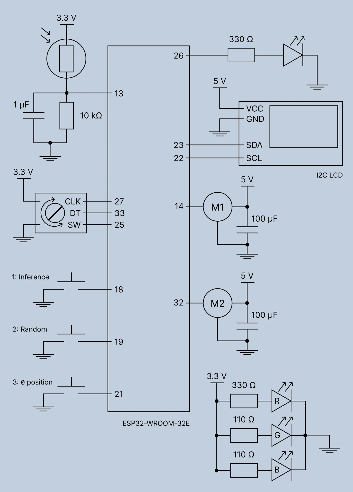
To assemble the circuit with the Adafruit HUZZAH32 Feather (ESP32-WROOM-32E) MCU board, the following pin mappings are used:

• Photoresistor (voltage divider):

  • Leg 1 → ESP32 3.3V
  • Leg 2 → voltage divider* → ESP32 GPIO 13 (A12)

  • The voltage divider is implemented by placing a 10 kΩ resistor between the photoresistor’s leg 2 and GND. This ensures that the voltage at GPIO 13 is proportional to the light intensity detected by the photoresistor.

• LED indicator:

  • Anode (long leg) → 330 Ω resistor → ESP32 GPIO 26 (A0)
  • Cathode (short leg) → ESP32 GND

• RGB LED (always ON):

  • Red → 330 Ω resistor → ESP32 3.3V
  • Green → 110 Ω resistor → ESP32 3.3V
  • Blue → 110 Ω resistor → ESP32 3.3V
  • Common Cathode → ESP32 GND

• Rotary encoder:

  • CLK → ESP32 GPIO 27
  • DT → ESP32 GPIO 33
  • SW (Push-button switch) → ESP32 GPIO 25
  • VCC → ESP32 3.3V
  • GND → ESP32 GND

• I2C LCD (16x2):

  • SDA → ESP32 GPIO 23
  • SCL → ESP32 GPIO 22
  • VCC → ESP32 USB pin (5V)
  • GND → ESP32 GND

• Servo motors (powered by a separate 5V supply):

  • Motor 1 (Pan) Signal → ESP32 GPIO 14
  • Motor 2 (Tilt) Signal → ESP32 GPIO 32

• Push Buttons (using internal pull-ups):

  • Button 1 (Inference): Leg 1 → ESP32 GPIO 18, Leg 2 → ESP32 GND
  • Button 2 (Random position): Leg 1 → ESP32 GPIO 19, Leg 2 → ESP32 GND
  • Button 3 (Position “0”): Leg 1 → ESP32 GPIO 21, Leg 2 → ESP32 GND

Power decoupling and noise filtering

To ensure high reliability, prevent microcontroller resets from motor voltage dips, and eliminate sensor noise, passive capacitors are distributed across the circuit as follows:

1. Servo motor power rail (bulk decoupling): 2 × 100 µF electrolytic capacitors are placed across the 5V motor power rails and GND, positioned physically close to the servos’power headers. In addition, a 10 µF electrolytic capacitor (not shown in the schematic) is placed between the 5V power input and GND where the 5V power enters the board. This configuration acts as a local energy reservoir to prevent voltage sag and system brownouts caused by sudden, massive current spikes drawn by the servos when actuating under load.

2. Photoresistor analog input (ADC Low-Pass Filter): a 1 µF electrolytic capacitor is connected in parallel with the 10 kΩ pull-down resistor between GPIO 13 and GND.This smooths out high-frequency noise from the ESP32 ADC and eliminates artificial room lighting flicker without delaying the sensor’s response to physical movement.

3. Rotary encoder (EMI suppression): 3 × 100 pF ceramic capacitors (not shown in the schematic) are connected between GND and the signal lines of sensitive switches (CLK, DT, SW) to suppress ultra-high-frequency electromagnetic interference (EMI) picked up by jumper wires from motor switching noise to ground.

Firmware

FreeRTOS tasks

The ESP32 controls the dual pan-tilt servo assembly, reads the light sensor, handles the rotary encoder, displays the status on the LCD, and executes the Q-learning grid-scan training and inference. All these responsibilities must be divided into independent tasks running concurrently to avoid blocking and keep the system responsive. This functionality is implemented using the FreeRTOS kernel that provides lightweight multitasking, thread scheduling based on priorities, inter-task communication, and precise timing on resource-constrained hardware.

The following functions and macros from FreeRTOS.h and task.h are used in the firmware:

• xTaskCreate(): spawns a new task thread with a specified stack size, priority, and entry function
• vTaskDelete(): terminates a task and frees its stack memory
• vTaskDelay(): suspends the calling task for a given number of OS ticks, yielding CPU time to other tasks
• xTaskGetTickCount(): returns the count of OS ticks elapsed since startup
• pdMS_TO_TICKS(): a macro that converts time in milliseconds into FreeRTOS tick units based on configTICK_RATE_HZ
• pdTICKS_TO_MS(): a macro that converts FreeRTOS ticks back into milliseconds
• portsTICK_PERIOD_MS: a constant defining the millisecond length of a single OS tick

The FreeRTOS tasks running on the MCU are shown in the diagram below.

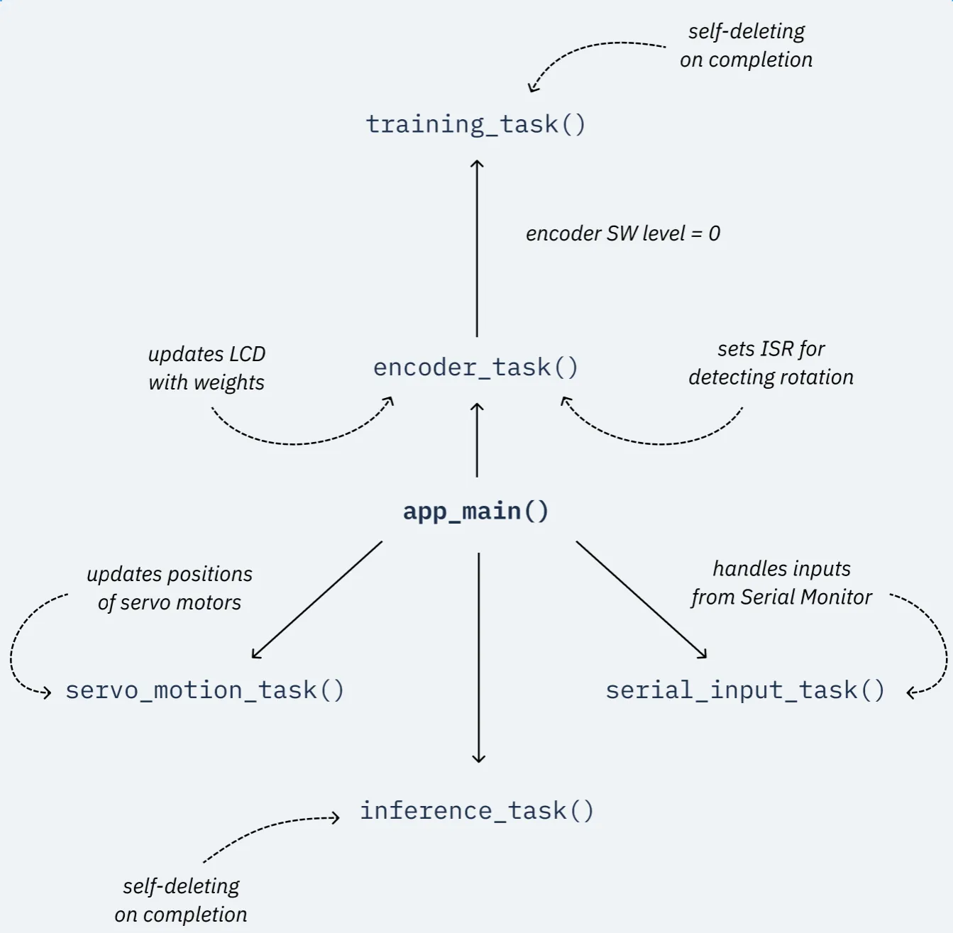
• servo_motion_task: Runs periodically at 50 Hz (every 20 ms). It calculates cosine ease-in/ease-out acceleration for the pan and tilt servos and updates PWM duty cycles smoothly without delaying other code:

void servo_motion_task(void *pvParameters) {
    while (1) {
        uint32_t now = pdTICKS_TO_MS(xTaskGetTickCount());
        
        for (int i = 0; i < 2; i++) {
            servo_state_t *s = &servos[i];
            if (s->is_moving) {
                uint32_t elapsed = now - s->start_time_ms;
                
                if (elapsed >= s->duration_ms) {
                    // Motion complete
                    s->current_angle = s->target_angle;
                    s->is_moving = false;
                    update_servo_hw(s->channel, s->current_angle);
                } else {
                    // Normalize time from 0.0 to 1.0
                    float t = (float)elapsed / (float)s->duration_ms;
                    
                    // Ease in-out using cosine
                    float ease_progress = (1.0f - cosf(M_PI * t)) / 2.0f;
                    
                    // Interpolate
                    s->current_angle = s->start_angle + (s->target_angle - s->start_angle) * ease_progress;
                    update_servo_hw(s->channel, s->current_angle);
                }
            }
        }
        vTaskDelay(pdMS_TO_TICKS(SERVO_UPDATE_PERIOD_MS));
    }
}

• encoder_task: Handles user input from the rotary encoder to tune reward weight parameters (weight_t and weight_v), updates the I2C LCD display, performs deferred saving to NVS after 3 seconds of inactivity, and listens for the encoder pushbutton to trigger Q-learning training:

void encoder_task(void *pvParameters) {
    // 1. Configure the GPIO pins
    gpio_config_t enc_config = {
        .pin_bit_mask = (1ULL << ENCODER_CLK_GPIO) | (1ULL << ENCODER_DT_GPIO) | (1ULL << ENCODER_SW_GPIO),
        .mode = GPIO_MODE_INPUT,
        .pull_up_en = GPIO_PULLUP_ENABLE,
        .pull_down_en = GPIO_PULLDOWN_DISABLE,
        .intr_type = GPIO_INTR_ANYEDGE // Trigger interrupt on any change to CLK
    };
    gpio_config(&enc_config);

    // 2. Install the GPIO ISR service and attach the handler to the CLK pin
    gpio_install_isr_service(0);
    last_clk_state = gpio_get_level(ENCODER_CLK_GPIO);
    gpio_isr_handler_add(ENCODER_CLK_GPIO, encoder_isr_handler, NULL);
    
    while (1) {
        // We only check if the interrupt has changed the value
        if (abs(encoder_value - last_encoder_value) >= 2) {
            if (encoder_value > last_encoder_value) {
                weight_t += 0.05f;
            } else {
                weight_t -= 0.05f;
            }
            
            if (weight_t > 1.0f) weight_t = 1.0f;
            if (weight_t < 0.0f) weight_t = 0.0f;
            
            weight_v = 1.0f - weight_t;
            last_encoder_value = encoder_value;
            
            update_lcd_display();
            
            // Mark for delayed saving
            weights_need_saving = true;
            last_knob_turn_time = xTaskGetTickCount() * portTICK_PERIOD_MS;
        }
        
        // Execute delayed save if 3 seconds have passed
        if (weights_need_saving) {
            uint32_t current_time = xTaskGetTickCount() * portTICK_PERIOD_MS;
            if (current_time - last_knob_turn_time >= 3000) {
                save_weights(weight_t);
                weights_need_saving = false;
            }
        }
        
        // Update LCD periodically with live sensor values (every ~500ms)
        static uint32_t last_lcd_update = 0;
        uint32_t current_time = xTaskGetTickCount() * portTICK_PERIOD_MS;
        if (current_time - last_lcd_update > 500) {
            update_lcd_display();
            last_lcd_update = current_time;
        }
        
        // Also check encoder switch
        if (gpio_get_level(ENCODER_SW_GPIO) == 0) {
            printf("\nEncoder Button Pressed! Wiping Q-table and starting training...\n");
            xTaskCreate(training_task, "training_task", 8192, NULL, 4, NULL);
            // Debounce
            vTaskDelay(pdMS_TO_TICKS(1000));
        }

        vTaskDelay(pdMS_TO_TICKS(50)); // Check for UI updates at a safe 20Hz
    }
}

• serial_input_task: Reads commands asynchronously over the UART serial monitor without blocking motor execution or UI rendering. This task allows the user to set the pan and tilt angles directly to calibrate the servos by issuing commands like p 90 for panning or t 45 for tilting:

void serial_input_task(void *pvParameters) {
    char input_buf[64];
    
    while (1) {
        printf("\nEnter command (p <angle> for Pan, t <angle> for Tilt): ");
        fflush(stdout);

        if (fgets(input_buf, sizeof(input_buf), stdin) != NULL) {
            input_buf[strcspn(input_buf, "\r\n")] = 0;
            
            if (strlen(input_buf) > 0) {
                char motor;
                float angle = 0;
                
                if (sscanf(input_buf, "%c %f", &motor, &angle) == 2) {
                    if (motor == 'p' || motor == 'P') {
                        printf("\nMoving Pan Servo to %.1f degrees smoothly.\n", angle);
                        set_servo_angle_smooth(PAN_SERVO_INDEX, angle);
                    } else if (motor == 't' || motor == 'T') {
                        printf("\nMoving Tilt Servo to %.1f degrees smoothly.\n", angle);
                        set_servo_angle_smooth(TILT_SERVO_INDEX, angle);
                    } else {
                        printf("\nError: Unknown motor. Use 'p' or 't'.\n");
                    }
                } else {
                    printf("\nError: Invalid format. Example: p 90\n");
                }
            }
        }
        vTaskDelay(pdMS_TO_TICKS(10)); 
    }
}

• training task: It is spawned on demand and executes the full Q-learning training (grid scanning pan/tilt positions, reading rewards, running 1000 value iteration updates, and saving results to NVS), deleting itself upon completion:

void training_task(void *pvParameters) {
    printf("\n--- STARTING TRAINING ---\n");
    gpio_set_level(LED_INDICATOR_GPIO, 0); // Turn off LED
    memset(q_table, 0, sizeof(q_table));
    memset(rewards_matrix, 0, sizeof(rewards_matrix));
    
    // 1. Grid Scan
    for (int pan = 0; pan < 12; pan++) {
        for (int tilt = 0; tilt < 12; tilt++) {
            // Move hardware
            set_servo_angle_smooth(PAN_SERVO_INDEX, pan * 15.0f);
            set_servo_angle_smooth(TILT_SERVO_INDEX, tilt * 15.0f);
            
            // Wait for motion to complete
            while (servos[PAN_SERVO_INDEX].is_moving || servos[TILT_SERVO_INDEX].is_moving) {
                vTaskDelay(pdMS_TO_TICKS(50));
            }
            // Extra settle time
            vTaskDelay(pdMS_TO_TICKS(100));
            
            // Calculate and store reward
            rewards_matrix[pan][tilt] = calculate_reward(tilt);
        }
    }
    
    printf("\nGrid scan complete. Running Value Iteration...\n");
    
    // 2. Value Iteration (in memory)
    float alpha = 0.1f;
    float gamma = 0.9f;
    
    for (int iter = 0; iter < 1000; iter++) {
        for (int pan = 0; pan < 12; pan++) {
            for (int tilt = 0; tilt < 12; tilt++) {
                for (int a = 0; a < 4; a++) { // 0=PAN_LEFT, 1=PAN_RIGHT, 2=TILT_UP, 3=TILT_DOWN
                    // Determine next state
                    int next_pan = pan;
                    int next_tilt = tilt;
                    if (a == 0 && pan > 0) next_pan--; // PAN_LEFT
                    if (a == 1 && pan < 11) next_pan++; // PAN_RIGHT
                    if (a == 2 && tilt > 0) next_tilt--; // TILT_UP (0 is up)
                    if (a == 3 && tilt < 11) next_tilt++; // TILT_DOWN (11 is down)
                    
                    // Find max Q in next state
                    float max_q_next = 0.0f;
                    for (int next_a = 0; next_a < 4; next_a++) {
                        if (q_table[next_pan][next_tilt][next_a] > max_q_next) {
                            max_q_next = q_table[next_pan][next_tilt][next_a];
                        }
                    }
                    
                    // Update Q-value
                    float r = rewards_matrix[next_pan][next_tilt];
                    q_table[pan][tilt][a] = q_table[pan][tilt][a] + alpha * (r + gamma * max_q_next - q_table[pan][tilt][a]);
                }
            }
        }
    }
    
    // 3. Print Q-table Max Values
    printf("\n--- OPTIMAL POLICY (Max Q-Values) ---\n");
    for (int tilt = 0; tilt < 12; tilt++) {
        for (int pan = 0; pan < 12; pan++) {
            float max_q = 0.0f;
            for (int a = 0; a < 4; a++) {
                if (q_table[pan][tilt][a] > max_q) {
                    max_q = q_table[pan][tilt][a];
                }
            }
            printf("%.2f ", max_q);
        }
        printf("\n");
    }
    
    // 4. Return to center
    set_servo_angle_smooth(PAN_SERVO_INDEX, 90.0f);
    set_servo_angle_smooth(TILT_SERVO_INDEX, 90.0f);
    
    // 5. Save to NVS
    save_q_table();
    
    printf("\nTraining complete!\n");
    gpio_set_level(LED_INDICATOR_GPIO, 1); // Turn on LED
    
    vTaskDelete(NULL);
}

• inference_task: It is spawned on demand and runs greedy navigation using the learned Q-table to navigate to the light source, deleting itself upon completion:

void inference_task(void *pvParameters) {
    printf("\n--- STARTING INFERENCE ---\n");
    bool visited[12][12];
    memset(visited, 0, sizeof(visited));
    
    while(1) {
        int pan = (int)(servos[PAN_SERVO_INDEX].target_angle / 15.0f + 0.5f);
        int tilt = (int)(servos[TILT_SERVO_INDEX].target_angle / 15.0f + 0.5f);
        
        // Safety bounds
        if (pan > 11) pan = 11; 
        if (pan < 0) pan = 0;
        if (tilt > 11) tilt = 11; 
        if (tilt < 0) tilt = 0;
        
        visited[pan][tilt] = true;
        
        // Find best action
        float max_q = -1.0f;
        int best_a = -1;
        
        for(int a=0; a<4; a++) {
            if(q_table[pan][tilt][a] > max_q) {
                max_q = q_table[pan][tilt][a];
                best_a = a;
            }
        }
        
        if (best_a == -1 || max_q == 0.0f) {
            printf("No valid path found (Q-table is likely empty).\n");
            break;
        }
        
        // Determine next state
        int next_pan = pan;
        int next_tilt = tilt;
        if (best_a == 0 && pan > 0) next_pan--; // PAN_LEFT
        if (best_a == 1 && pan < 11) next_pan++; // PAN_RIGHT
        if (best_a == 2 && tilt > 0) next_tilt--; // TILT_UP
        if (best_a == 3 && tilt < 11) next_tilt++; // TILT_DOWN
        
        if (next_pan == pan && next_tilt == tilt) {
            printf("Reached a wall. Destination found!\n");
            break;
        }
        
        // Loop prevention
        if (visited[next_pan][next_tilt]) {
            printf("Oscillation detected (peak reached). Destination found!\n");
            break;
        }
        
        // Execute move
        printf("Taking action %d (Q: %.2f) to [%d, %d]\n", best_a, max_q, next_pan, next_tilt);
        set_servo_angle_smooth(PAN_SERVO_INDEX, next_pan * 15.0f);
        set_servo_angle_smooth(TILT_SERVO_INDEX, next_tilt * 15.0f);
        
        // Wait for move to finish
        while (servos[PAN_SERVO_INDEX].is_moving || servos[TILT_SERVO_INDEX].is_moving) {
            vTaskDelay(pdMS_TO_TICKS(50));
        }
        vTaskDelay(pdMS_TO_TICKS(250)); // Brief pause before next step
    }
    
    printf("Inference complete.\n");
    vTaskDelete(NULL);
}

The main entry function app_main() is itself launched inside its own FreeRTOS task. It initialises GPIOs, the non-volatile storage (NVS) for the reward function weights and the Q-table, the sensor, the servo motors, and the I2C LCD, then creates background tasks and polls push-buttons:

void app_main(void) {
    // --- Configuring the Serial Monitor here --- //
    // --- ... --- //

    // 1. Configure Buttons (Button 1, 2 and 3) and LED
    gpio_config_t btn_config = {
        .pin_bit_mask = (1ULL << BUTTON_1_GPIO) | (1ULL << BUTTON_2_GPIO) | (1ULL << BUTTON_3_GPIO),
        .mode = GPIO_MODE_INPUT,
        .pull_up_en = GPIO_PULLUP_ENABLE,
        .pull_down_en = GPIO_PULLDOWN_DISABLE,
        .intr_type = GPIO_INTR_DISABLE
    };
    gpio_config(&btn_config);
    
    gpio_config_t led_config = {
        .pin_bit_mask = (1ULL << LED_INDICATOR_GPIO),
        .mode = GPIO_MODE_OUTPUT,
        .pull_up_en = GPIO_PULLUP_DISABLE,
        .pull_down_en = GPIO_PULLDOWN_DISABLE,
        .intr_type = GPIO_INTR_DISABLE
    };
    gpio_config(&led_config);
    gpio_set_level(LED_INDICATOR_GPIO, 0); // Initially off

    // --- Steps 2-5: Initialising NVS, loading weights and Q-table, initialising sensors, servos, I2C and LCD --- //
    // --- ... --- //

    // 6. Start Tasks
    xTaskCreate(servo_motion_task, "servo_motion_task", 4096, NULL, 5, NULL);
    xTaskCreate(serial_input_task, "serial_input_task", 4096, NULL, 5, NULL);
    xTaskCreate(encoder_task, "encoder_task", 4096, NULL, 5, NULL);

    printf("\nInitialization complete. Ready for Training or Inference.\n");

    // 6. Main loop to poll the buttons
    while (1) {
        if (gpio_get_level(BUTTON_1_GPIO) == 0) {
            printf("\nButton 1 pressed! Starting Inference...\n");
            xTaskCreate(inference_task, "inference_task", 4096, NULL, 5, NULL);
            vTaskDelay(pdMS_TO_TICKS(1000));
        }
        
        if (gpio_get_level(BUTTON_3_GPIO) == 0) {
            printf("\nButton 3 pressed! Setting motors to position 0 smoothly.\n");
            set_servo_angle_smooth(PAN_SERVO_INDEX, 0.0f);
            set_servo_angle_smooth(TILT_SERVO_INDEX, 0.0f);
            vTaskDelay(pdMS_TO_TICKS(200)); 
        }
        
        if (gpio_get_level(BUTTON_2_GPIO) == 0) {
            // Generate random angles within the operational range
            float rand_pan = (float)(esp_random() % (int)(SERVO_MAX_DEGREE + 1));
            float rand_tilt = (float)(esp_random() % (int)(SERVO_MAX_DEGREE + 1));
            
            printf("\nButton 2 pressed! Randomizing motors smoothly: Pan=%.1f, Tilt=%.1f\n", rand_pan, rand_tilt);
            set_servo_angle_smooth(PAN_SERVO_INDEX, rand_pan);
            set_servo_angle_smooth(TILT_SERVO_INDEX, rand_tilt);
            vTaskDelay(pdMS_TO_TICKS(200)); 
        }

        vTaskDelay(pdMS_TO_TICKS(10));
    }
}

Without FreeRTOS, running motor easing, reading serial commands, polling buttons, updating an LCD, and running training algorithms would block each other or require complex state machines. This firmware uses several RTOS design patterns to ensure non-blocking concurrent execution:

1. Cooperative Yielding with vTaskDelay(): In FreeRTOS, if a task runs an infinite while(1) loop without yielding, it will starve other equal or lower priority tasks and trigger the ESP32 Task Watchdog Timer reset. This is why every task loop contains an explicit vTaskDelay(...) call. FreeRTOS then moves the task to the Blocked state, consuming 0% CPU cycles until its delay expires. This leaves the CPU completely free for other tasks.

2. Task Priority Hierarchy: Tasks are assigned numerical priorities during xTaskCreate()(higher number = higher priority):

• servo_motion_task, serial_input_task, encoder_task, inference_task: Priority 5 (High responsiveness for motion, serial, and UI).
• training_task: Priority 4 (Slightly lower priority so that heavy computational matrix calculations do not starve UI or motor updates).

3. Asynchronous Background Task Delegation: When the user presses the Encoder button to start training or Button 1 to run inference, the system doesn’t execute training directly inside the UI loop. Instead, it calls xTaskCreate(training_task, ...) to spawn training on a separate thread with its own 8KB stack. The UI loop immediately continues without freezing. Once training finishes, training_task calls vTaskDelete(NULL) to destroy itself and free memory.

4. Non-Blocking Servo Easing: Calling set_servo_angle_smooth() does not wait 3 seconds for the motor to finish moving. It simply records the target angle and start timestamp in a shared global struct. The dedicated servo_motion_task wakes up every 20 ms in the background to calculate the next position along a cosine curve and update PWM hardware.

typedef struct {
  int channel;
  float current_angle;
  float start_angle;
  float target_angle;
  uint32_t start_time_ms;
  uint32_t duration_ms;
  bool is_moving;
} servo_state_t;

// Global state for servos
servo_state_t servos[2];

5. ISR + Deferred Processing for Encoder: Rotary encoder pulses are handled via an Interrupt Service Routine (encoder_isr_handler) attached to the CLK pin. The ISR executes in microseconds to update encoder_value, while encoder_task periodically reads the value and updates the LCD display without blocking any hardware operations.

static void IRAM_ATTR encoder_isr_handler(void* arg) {
  uint8_t clk = gpio_get_level(ENCODER_CLK_GPIO);
  uint8_t dt = gpio_get_level(ENCODER_DT_GPIO);
  
  if (clk != last_clk_state) {
      if (dt != clk) {
          encoder_value++;
      } else {
          encoder_value--;
      }
      last_clk_state = clk;
  }
}

Servo motors’ smooth movement

Both servo motors are driving heavy steel platforms with a high moment of inertia. To prevent damage to the hardware, the servo logic implements the smooth ease-in/ease-out motion using a cosine function.

void servo_motion_task(void *pvParameters) {
    while (1) {
        uint32_t now = pdTICKS_TO_MS(xTaskGetTickCount());
        
        for (int i = 0; i < 2; i++) {
            servo_state_t *s = &servos[i];
            if (s->is_moving) {
                uint32_t elapsed = now - s->start_time_ms;
                
                if (elapsed >= s->duration_ms) {
                    // Motion complete
                    s->current_angle = s->target_angle;
                    s->is_moving = false;
                    update_servo_hw(s->channel, s->current_angle);
                } else {
                    // Normalize time from 0.0 to 1.0
                    float t = (float)elapsed / (float)s->duration_ms;
                    
                    // Ease in-out using cosine
                    float ease_progress = (1.0f - cosf(M_PI * t)) / 2.0f;
                    
                    // Interpolate
                    s->current_angle = s->start_angle + (s->target_angle - s->start_angle) * ease_progress;
                    update_servo_hw(s->channel, s->current_angle);
                }
            }
        }
        vTaskDelay(pdMS_TO_TICKS(SERVO_UPDATE_PERIOD_MS));
    }
}

The API for requesting a smooth motion handles motion thresholds and sets the motion duration based on the distance to travel based on the estimate of 3 seconds for the full 165° range of the servo.

void set_servo_angle_smooth(int servo_index, float target_angle) {
    if (servo_index < 0 || servo_index > 1) return;
    if (target_angle < 0.0f) target_angle = 0.0f;
    if (target_angle > SERVO_MAX_DEGREE) target_angle = SERVO_MAX_DEGREE;
    
    servo_state_t *s = &servos[servo_index];
    
    // If we're already close, don't bother moving
    if (fabs(target_angle - s->current_angle) < 0.1f) return;

    s->start_angle = s->current_angle;
    s->target_angle = target_angle;
    s->start_time_ms = pdTICKS_TO_MS(xTaskGetTickCount());
    
    // Scale duration based on distance to move (3000ms for full 165 degrees)
    float distance = fabs(target_angle - s->start_angle);
    s->duration_ms = (uint32_t)((distance / SERVO_MAX_DEGREE) * MOTION_FULL_RANGE_MS);
    
    // Handle very short durations to avoid div by zero
    if (s->duration_ms < SERVO_UPDATE_PERIOD_MS) {
        s->duration_ms = SERVO_UPDATE_PERIOD_MS;
    }
    
    s->is_moving = true;
}

Experiment walkthrough

The experiment is divided into two phases: training and inference. The training phase involves scanning the entire pan-tilt grid, calculating rewards, and filling the Q-table. The inference phase uses the learned Q-table to navigate towards the light source.

Training

Before the training begins, the exising Q-table stored in the non-volatile storage (NVS) is wiped to ensure that the robot starts with a clean slate. The training is conducted for the pre-defined position of the light source and with the current reward function weights. In other words, Q-table is specific to the current environment and reward function configuration. If the light source is moved or the reward function weights are changed, the Q-table must be retrained.

Filling the Q-table

The Q-table is implemented as a 3D array of floats, where the first two dimensions represent the discretized pan and tilt positions (12 each), and the third dimension are the four possible actions (PAN_LEFT, PAN_RIGHT, TILT_UP, TILT_DOWN).

float q_table[12][12][4]; 

At the training phase, the Q-table is filled based on the reward matrix values collected during the grid scan.

for (int pan = 0; pan < 12; pan++) {
        for (int tilt = 0; tilt < 12; tilt++) {
            // Move hardware
            set_servo_angle_smooth(PAN_SERVO_INDEX, pan * 15.0f);
            set_servo_angle_smooth(TILT_SERVO_INDEX, tilt * 15.0f);
            
            // Wait for motion to complete
            while (servos[PAN_SERVO_INDEX].is_moving || servos[TILT_SERVO_INDEX].is_moving) {
                vTaskDelay(pdMS_TO_TICKS(50));
            }
            // Extra settle time
            vTaskDelay(pdMS_TO_TICKS(100));
            
            // Calculate and store reward
            rewards_matrix[pan][tilt] = calculate_reward(tilt);
        }
    }
    
    // 2. Value Iteration (in memory)
    float alpha = 0.1f;
    float gamma = 0.9f;
    
    for (int iter = 0; iter < 1000; iter++) {
        for (int pan = 0; pan < 12; pan++) {
            for (int tilt = 0; tilt < 12; tilt++) {
                for (int a = 0; a < 4; a++) { // 0=PAN_LEFT, 1=PAN_RIGHT, 2=TILT_UP, 3=TILT_DOWN
                    // Determine next state
                    int next_pan = pan;
                    int next_tilt = tilt;
                    if (a == 0 && pan > 0) next_pan--; // PAN_LEFT
                    if (a == 1 && pan < 11) next_pan++; // PAN_RIGHT
                    if (a == 2 && tilt > 0) next_tilt--; // TILT_UP (0 is up)
                    if (a == 3 && tilt < 11) next_tilt++; // TILT_DOWN (11 is down)
                    
                    // Find max Q in next state
                    float max_q_next = 0.0f;
                    for (int next_a = 0; next_a < 4; next_a++) {
                        if (q_table[next_pan][next_tilt][next_a] > max_q_next) {
                            max_q_next = q_table[next_pan][next_tilt][next_a];
                        }
                    }
                    
                    // Update Q-value
                    float r = rewards_matrix[next_pan][next_tilt];
                    q_table[pan][tilt][a] = q_table[pan][tilt][a] + alpha * (r + gamma * max_q_next - q_table[pan][tilt][a]);
                }
            }
        }
    }

Note that this algorithm is a mathematical simulation rather than the original model-free Q-learning. In a traditional Q-learning algorithm, the agent does not know the layout of the environment and rewards for each action in advance.They are learned by trial and error by taking an action, observing the resulting reward, and updating the Q-value for that specific state-action pair. The current implementation bypasses the learning process by first systematically visiting every single state (all 144 grid positions) and recording the exact reward in the rewards_matrix. Because the transition model is fully known and deterministic, the code then runs a nested loop for 1000 iterations purely in memory. It mathematically simulates moving around the environment to propagate the rewards through the Q-table without the physical motion.

The implementation of true tabular Q-learning would involve episodic exploration, where the robot, instead of a neat row-by-row scan, starts at a random position, takes random actions, and updates the Q-table based on the observed rewards. This would require thousands of physical steps to converge, making the robot wander around pseudo-randomly for hours. Besides the time factor, the risk of incomplete knowledge would affect the quality of inference if the robot does not explore all possible chains of states.

After the training is complete, the Q-table is saved to non-volatile storage (NVS) so that it can be used later for inference without retraining. A snapshot of the Q-table’s maximum values is printed to the serial monitor for debugging and verification.

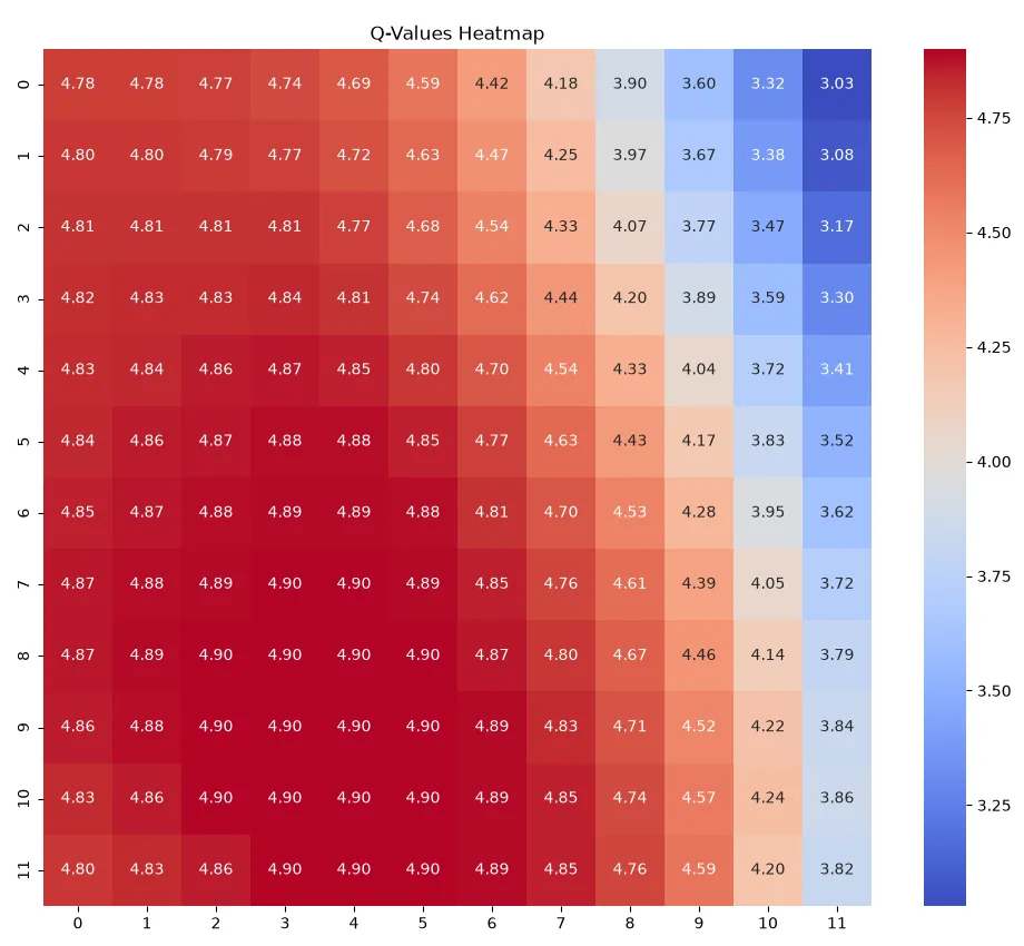
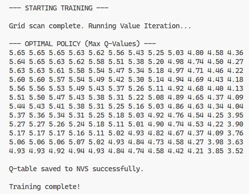
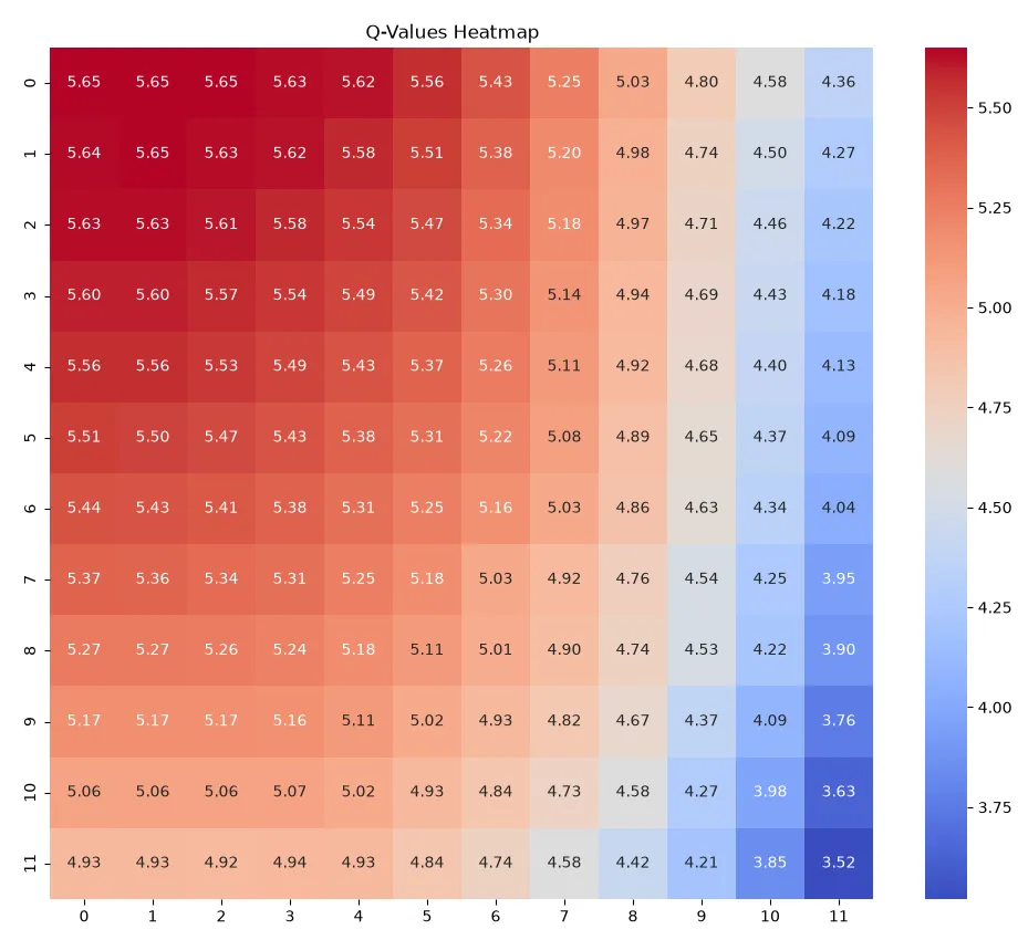
Below you can see two sample Q-table snapshots printed to the serial monitor after training with different reward function weights.

The first snapshot shows a Q-table trained with weight_t=0.0 and weight_v=1.0 – the one that resulted in the robot “reward hacking” by pointing down to the local light source that maximized the reward.

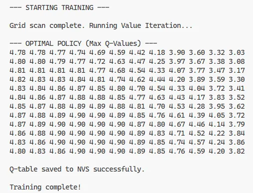
The second snapshot is the result of an attempt to counteract the reward hacking by adjusting the weights to weight_t=0.2 and weight_v=0.0 that slightly increases the reward when the robot tilts the sensor up.

Inference

At the inference phase, the robot uses the learned Q-table to navigate towards the light source until the reward value starts oscillating, indicating that it has reached a local maximum, as observed when the tilt value is set to 0.0…

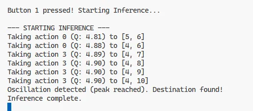
…or when the edge of the grid is reached, as observed when the tilt value is set to 0.2.

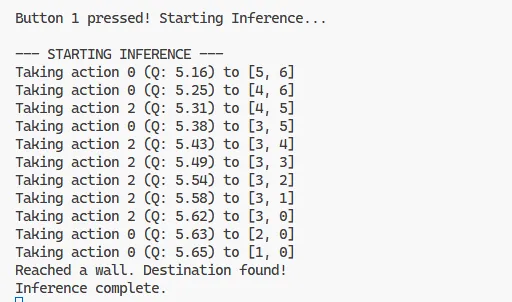
Rather than executing a simple “pan all the way, then tilt” strategy, the Light Seeker takes an intricate, zigzagging trajectory towards the target. This behaviour is a manifestation of the agent performing gradient ascent on the Q-value landscape. At any given state, the Q-learning policy ($\pi(s) = \arg\max_a Q(s,a)$) forces it to evaluate its immediate surroundings and choose the step that maximizes its cumulative discounted future reward.

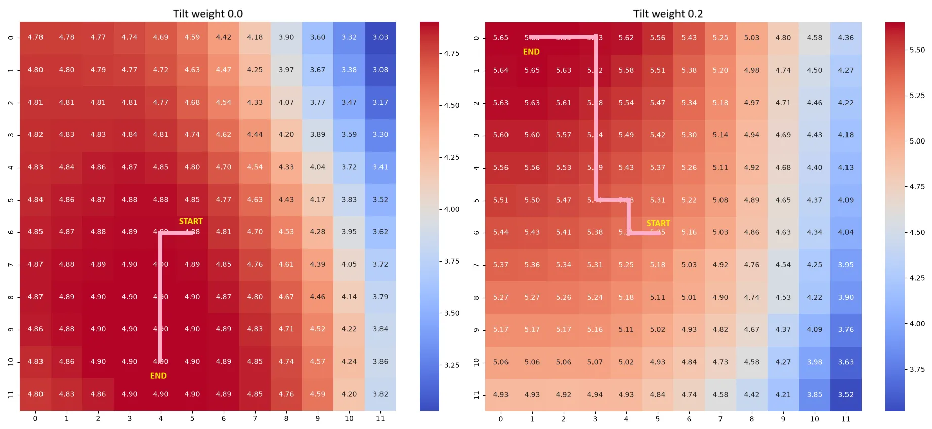
Crucially, despite taking this intricate path, the robot never takes a trajectory that is longer than strictly necessary. This efficiency is enforced by the discount factor ($\gamma$) in the Bellman equation: $Q(s,a) = R(s') + \gamma \max_{a'} Q(s',a')$.

Because $\gamma$ is set to a value strictly less than $1.0$ (in this case, $\gamma = 0.9$), future rewards exponentially decay the further away they are in time (i.e. the longer the path). Reaching the absolute peak reward in 5 steps yields a significantly higher cumulative Q-value than reaching it in 6 steps ($0.9^5 > 0.9^6$). Consequently, the mathematical optimisation inherently penalises taking unnecessarily long paths, guaranteeing that the Seeker’s intricate trajectory is always the most mathematically direct route to the global maximum.

A note on greedy inference

The Light Seeker performs greedy inference during the navigation phase, meaning that at each step it selects the action with the highest Q-value for its current state. This is implemented in the inference_task as follows:

src/main.c

// Find best action
float max_q = -1.0f;
int best_a = -1;

for(int a=0; a<4; a++) {
    if(q_table[pan][tilt][a] > max_q) {
        max_q = q_table[pan][tilt][a];
        best_a = a;
    }
}

Listing 14. Greedy inference task: navigating to the light source using the learned Q-table

It does not plan multiple steps ahead or explore alternative routes; it simply performs gradient ascent by stepping toward the highest adjacent Q-value, trusting that the training phase correctly encoded the optimal long-term path into those values.

Tabular Q-learning is, therefore, an eager learning method. It spends computational time up front during training to built a complete Q-table, making the inference phase fast and lightweight, implemented here as a simple array lookup. A lazy learning algorithm would be inference-heavy: to decide where to move, the agent would have to calculate the optimal path on the fly. In an embedded system, eager learning with greedy inference guarantees that the MCU can instantly look up the next move, resulting in smooth, continuous physical motion.

Conclusion

The Light Seeker serves as a tangible demonstration of the proxy alignment problem and reward hacking in reinforcement learning. By exposing how an agent will ruthlessly optimise for a flawed proxy metric (the raw voltage from a nearby LED) over the true objective (ambient light energy), it highlights a fundamental challenge in AI safety and system design.

However, it is important to note that while this experiment is framed as an imitation of a solar panel, the suggested Q-learning approach is not suitable for a real-world solar panel installation. The tabular Q-learning implementation here assumes a static environment. In reality, the Sun moves continuously across the sky. Because the optimal state changes throughout the day, the agent would have to constantly re-learn the environment, rendering a static, episodic Q-table approach highly inefficient. Real solar tracking systems typically rely on deterministic astronomical algorithms (calculating the sun’s exact position based on time and GPS coordinates) or active closed-loop feedback (using paired light sensors to balance shading) rather than exploratory reinforcement learning.

Beyond the primary demonstration of Goodhart’s Law, the project yields several valuable pedagogical and technical insights:

• Multi-objective reinforcement learning: The fix to the reward hacking issue transforms the system into a multi-objective RL problem. By normalising both the sensor voltage and the physical tilt index to a common 0.0 to 1.0 scale, the agent is forced to balance competing goals.

• The “attention budget” and reward bounding: Constraining the weights to sum to 1 provides a clear visual representation of trade-offs (e.g., 80% proxy vs. 20% spatial orientation) while simultaneously ensuring mathematical stability. Bounding the maximum reward prevents wild Q-value inflation, keeping the learning rate ($\alpha$) and discount factor ($\gamma$) stable across different weight configurations.

• The curse of dimensionality: The project illustrates the limitations of tabular Q-Learning. While a 12x12 grid easily fits into the ESP32’s memory, increasing spatial granularity or adding a third axis would cause the state-action table to explode. Scaling this to a continuous state space would require a paradigm shift to Deep Q-learning (DQN) and likely necessitate offloading the neural network computations to an edge server due to the microcontroller’s constraints.

• Hardware and software symbiosis: Running RL algorithms on physical hardware introduces challenges that don’t exist in simulations. The firmware successfully navigates this by utilising FreeRTOS for concurrent, non-blocking tasks (separating the UI, serial inputs, and motor control) and employing software-defined boundary constraints and hysteresis-like movement thresholds to prevent motor burnout and mechanical jitter during the exploratory value iterations.

Ultimately, the Light Seeker bridges the gap between abstract AI safety theories and applied embedded engineering, proving that even a microcontroller with 2.25 KB of memory dedicated to a lookup table can fall victim to the exact same alignment failures as massive, state-of-the-art AI models.